Numeric control

Hint: When magnetic field is switched on (only 2D and 3D), the 1-band Schrödinger equation will be solved with a complex eigenvalue solver.
However, if the magnetic field strength is zero, all imaginary entries are zero.
In that case, a real eigenvalue solver would be faster.
Exactly, the same applies for the superlattice option.
You could specify "magnetic-field-on = yes" and "magnetic-field-strength = 0.0d0"(keyword $magnetic-field) in order to solve the 1-band Schrödinger equation with the complex method rather than using the real solvers.

Cutoff for Schrödinger equation eigenvalue solver

schroedinger-chearn-el-cutoff = 5d0   ! [eV] 2D/3D
schroedinger-chearn-hl-cutoff = 5d0   ! [eV] 2D/3D

Relative cutoff for Chebychev-Arnoldi eigenvalue solver in units of [eV].
Reference is the minimum band edge for electrons and the maximum band edge for holes.
Absolute band edge for electrons: Minimum band edge for electrons + schroedinger-chearn-el-cutoff
Absolute band edge for holes:      Maximum band edge for holes       - schroedinger-chearn-hl-cutoff
Note: This parameter is also necessary for the FEAST eigenvalue solver.
 

6x6 and 8x8 k.p Schrödinger equation

Eigenvalue solver option for 6x6 and 8x8 k.p Schrödinger equation:

schroedinger-kp-ev-solv     = lapack               ! 1D
                            = LAPACK-ZHEEV         ! 1D
                            = LAPACK-ZHEEVX        ! 1D
                            = laband               ! 1D/2D/3D
                            = LAPACK-ZHBGV         ! 1D/2D/3D
                            = LAPACK-ZHBGVX        ! 1D/2D/3D
                            = arpack               ! 1D/2D/3D
                            = arpack-shift-invert  !      2D/3D
                            = chearn               ! 1D/2D/3D
                            = it_jam               ! 1D/2D/3D
                            = FEASTd               ! 1D (FEAST-dense)
lapack        = ZHEEV  from LAPACK package (calculates all eigenvalues)
LAPACK-ZHEEV  = ZHEEV  from LAPACK package (calculates all eigenvalues)
                1D default
                2D not implemented
                3D not implemented
LAPACK-ZHEEVX = ZHEEVX from LAPACK package (calculates selected eigenvalues thus faster than lapack)
                1D default
                2D/3D not implemented
laband        = ZHBGV  from LAPACK package for banded matrix (1D)
LAPACK-ZHBGV  = ZHBGV  from LAPACK package for banded matrix (1D)
                ZHBGVX from LAPACK package for banded matrix (2D/3D) for schroedinger-kp-discretization = box-integration only
LAPACK-ZHBGVX = ZHBGVX from LAPACK package for banded matrix
                2D/3D for schroedinger-kp-discretization = box-integration only
arpack        = Arnoldi from ARPACK package with option
                'SM' ! smallest magnitude      (8x8 k.p, for holes and electrons) (complex version)
                'LR' !   largest real parts        (6x6 k.p, for holes)                     (complex version)
arpack-shift-invert =
                Arnoldi from ARPACK package with option
                1D not tested yet
                2D/3D not tested yet
chearn        = Chebychev-Arnoldi (Arnoldi form with Chebychev preconditioning)
                (eigenvalue solver for hermitian matrices)
                1D
                2D
                3D
it_jam        = iterative method by Jacek Majewski (not tested sufficiently)
                Only for extreme eigenvalues if inner eigenvalue H² is diagonalized.
                1D not tested yet
                2D not tested yet
                3D not tested yet
FEASTd        = FEAST dense solver
                FEAST solver package:
                E. Polizzi, Density-Matrix-Based Algorithms for Solving Eigenvalue Problems, Phys. Rev. B 79, 115112 (2009)
                Note: FEAST requires an upper limit where to search for eigenvalues, similar to 'chearn'.
 

Note, for 6x6 k.p in 2D and 3D it is recommended to use arpack. In 1D, lapack should be used in all cases unless the matrices are larger than dimension = 1000.
The fastest results are obtained with chearn provided that the user sets the cutoff energy appropriately. Note that chearn does not work for 8x8 k.p where interior eigenvalues have to be calculated.

Some suggestions for the parameters:

• it_jam

schroedinger-kp-iterations   =          ! 1D
schroedinger-kp-iterations   =  30      ! 2D
schroedinger-kp-iterations   =          ! 3D
 ---> SchroedingerkpIterations1D (2D/3D)

schroedinger-kp-residual     =          ! 1D (value is a guess, needs some testing)
schroedinger-kp-residual     =  1.0d-10 ! 2D
schroedinger-kp-residual     =          ! 3D
 ---> SchroedingerkpResidual1D (2D/3D)

! itere_max = 30
! eps_itere = 1.0d-10
! itsub_max = 200
! eps_itsub = 1.0d-10

• Arnoldi
• Chebychev-Arnoldi
  => You will need a cutoff for the Schrödinger equation eigenvalue solver (see there for details):
     schroedinger-chearn-el-cutoff = 5d0
   schroedinger-chearn-hl-cutoff = 5d0

Eigensolver: arnoldi-complex
for 6x6 k.p or 8x8 k.p, i.e. Hermitian version
 
SchroedingerkpIterations1D (2D/3D) --> number of iterations
Set to a default value, does not change during simulation.
SchroedingerkpResidual1D (2D/3D)   --> precision for arnoldi method; is defined according to precision of outer loop

Note: For extreme eigenvalues --> arnoldi with option 'LM' or 'SM'
         For inner eigenvalues       --> arnoldi with option 'SM'

NOTE: All eigenvalues around E_separate are calculated due to H --> H-E_separate.
For electrons, however, one only needs eigenvalues above this edge (holes: below).
--> Number of eigenvalues is multiplied with a factor mult_num_ev_arnoldi and only the relevant eigenvalues are taken. mult_num_ev_arnoldi here is just a default value, it is specified in each k.p region.
If the calculated eigenvalues are not sufficient --> mult_num_ev_arnoldi (in the k.p region) is increased by add_num_ev_arnoldi, otherwise decreased by dec_num_ev_arnoldi.
If the calculated eigenvalues are not sufficient, H --> H-highest_eigenvalue and again the specified number of eigenvalues is calculated...

Note: arnoldi seems to have problems with degeneracies:
--> disturb_arnoldi is added to diagonal elements of the upper block in order to destroy the symmetry.

This currently applies only to: arpack
schroedinger-kp-more-ev    =  ?     ! 1D not implemented
schroedinger-kp-more-ev    =  5     ! 2D
schroedinger-kp-more-ev    =  5     ! 3D

schroedinger-kp-more-ev    =
  SchroedingerkpMoreEV1D/2D/3D --> If x eigenvalues are required, then arnoldi is asked to
                                   calculate x+delta_num_ev eigenvalues.
                                   This helps to improve convergence of eigenvalues. (Very often some eigenvalues are zero.)

schroedinger-kp-discretization = box-integration     ! 1D/2D/3D
                               = finite-differences  ! 1D/2D/3D (default)
Switch between box integration and finite differences discretization of k.p Schrödinger equation (similar to 1-band Schrödinger equation).

Schrödinger-Poisson problem

For coupled Schrödinger-Poisson equation.

schroedinger-poisson-problem       = precor  ! (predictor-corrector)
                                   = newton  ! not implemented yet
'precor' --> Predictor-corrector approach (default, only option so far)
'newton' --> Newton method is used (not implemented yet)
 

For predictor-corrector method

Number of iterations for Schrödinger-Poisson predictor-corrector cycle:

 schroedinger-poisson-precor-iterations = 12      ! 1D
 schroedinger-poisson-precor-iterations = 12      ! 2D
 schroedinger-poisson-precor-iterations = 12      ! 3D
 

Final precision for Schrödinger-Poisson predictor-corrector cycle:

 schroedinger-poisson-precor-residual   = 1.0d-9  ! 1D
 schroedinger-poisson-precor-residual   = 1.0d-9  ! 2D
 schroedinger-poisson-precor-residual   = 1.0d-9  ! 3D
                                        = 1.0d-16 ! 3D ???
 

SchroedingerPoissonPreCorIterXD  --> default value (default: 12)
SchroedingerPoissonPreCorResidXD --> default value (default: 1.0d-9)
Maybe introduce later a variable for these that change during execution.

Boundary conditions for Poisson equation along x, y and z directions

poisson-boundary-condition-along-x = periodic  !
                                   = Neumann   ! Neumann boundary conditions (default)
                                   = Dirichlet ! not implemented yet
poisson-boundary-condition-along-y = periodic  !
                                   = Neumann   ! Neumann boundary conditions (default)
                                   = Dirichlet ! not implemented yet
poisson-boundary-condition-along-z = periodic  !
                                   = Neumann   ! Neumann boundary conditions (default)
                                   = Dirichlet ! not implemented yet

This feature is useful if one has a superlattice and wants to have periodic boundary condtions for the Poisson equation as well.
It currently only works in 1D and 3D if the Poisson equation is solved over the whole device, i.e. contacts ($poisson-boundary-conditions) are not allowed.

Scale Poisson

scale-poisson = 1.0d0    ! 1D  (default: 1.0d0)
scale-poisson = 1.0d9    ! 2D  (default: 1.0d9)
scale-poisson = 1.0d18   ! 3D  (default: 1.0d18)

(Variable in code: ScalePoissonXD = 1.0d0)

In 1D the Poisson problem is scaled by 1.
In 3D and 2D the Poisson problem is scaled, as described in MODULE control_numeric:

Linear Poisson:
------------
Note: Using SI system has the effect that in equation

         PoissonM * xV = bV

both sides (i.e. PoissonM and bV) are scaled by a factor about 10^-22 in 3D (2D: 10^-12).
We have noticed that the conjugate gradient method in templates does not work well within that regime.
Therefore both sides are scaled by a factor ScalePoisson3D.
To be specific, all elements of PoissonM and bV are scaled AFTER definition of Dirichlet boundary conditions in subroutine scale_poisson.
ScalePoisson3D=1d18 has been proved to be adequate in 3D (2D: 1d9).
This value should not be altered.

Scale current

scale-current = 1.0d0    ! 1D  (default: 1.0d0)
scale-current = 1.0d0    ! 2D  (default: 1.0d0)
scale-current = 1.0d0    ! 3D  (default: 1.0d0)

(Variable in code: ScaleCurrentXD = 1.0d0)

Evaluation of Fermi functions (Fermi-Dirac integrals)

Note: Aymerich-Humet and vanHalen-Pulfrey are not implemented any more, so Trellakis is the default. Goano is possible, however.

fermi-function-mode = Trellakis         ! ='4'  Trellakis
                    = Goano             ! ='3'  Goano: Uses algorithm of Goano
                    = vanHalen-Pulfrey  ! ='2'  van Halen, Pulfrey: Uses approximations as documented in MODULE fermi_functions.
                    = Aymerich-Humet    ! ='1'  Aymerich-Humet
                   
FermiFunctionMode1D = '4' ! 'Trellakis' ! 1D (default)
FermiFunctionMode2D = '4' ! 'Trellakis' ! 2D (default)
FermiFunctionMode3D = '4' ! 'Trellakis' ! 3D (default)


fermi-function-precision = 1.0d-6  ! 1D
fermi-function-precision = 1.0d-6  ! 2D
fermi-function-precision = 1.0d-6  ! 3D

FermiFunctionPrecision1D/2D/3D --> only valid for 'Goano'
In case no approximation exists, 'Goano' is taken with FermiFunctionPrecision1D/2D/3D.

Not implemented yet:
Given are default values, they may be overwritten during execution. Defaults which are not changed during execution:
- FermiFunctionMode1D/2D/3D_default
- FermiFunctionPrecision1D/2D/3D_default

The following Fermi-Dirac integrals are used inside the code:
- F_3/2: - Goano (if (ABS(x) > 353.6d0) .AND. (ABS(x) < 354.2d0) Trellakis is used)
         (The calculation for ABS(x) from 353.6 up to 354.2 fails with Goano on SUN.)
       - Trellakis
- F_1/2: - Goano (if (ABS(x) > 353.6d0) .AND. (ABS(x) < 354.2d0) Trellakis is used)
         (The calculation for ABS(x) from 353.6 up to 354.2 fails with Goano on SUN.)
       - Trellakis
- F_-1/2: - Goano (if (ABS(x) > 353.6d0) .AND. (ABS(x) < 354.2d0) Trellakis is used)
         (The calculation for ABS(x) from 353.6 up to 354.2 fails with Goano on SUN.)
       - Trellakis
- F_-3/2: - Goano (if (ABS(x) > 353.6d0) .AND. (ABS(x) < 354.2d0) Trellakis is used)
         (The calculation for ABS(x) from 353.6 up to 354.2 fails with Goano on SUN.)
       - Trellakis

Allocate auxiliary Poisson matrix (number of offdiagonal elements)

Define variable for setting up auxiliary matrix. Then allocate storage for auxiliary matrix (modified sparse row storage format, actually COO formate so far). This is necessary if one performs 2D or 3D calculations and if one doesn't have enough memory. Then one could reduce the default value of memory allocation for the 2D or 3D Poisson matrix.

 poisson-allocate-auxiliary-matrix = (lengvecV)   ! 1D not applicable (full matrix is allocated)
 poisson-allocate-auxiliary-matrix = 500000       ! 2D
 poisson-allocate-auxiliary-matrix = 5000000      ! 3D

This number refers to the number of off-diagonal matrix elements.

Allocate auxiliary current matrix (number of offdiagonal elements)

Define variable for setting up auxiliary matrix. Then allocate storage for auxiliary matrix (modified sparse row storage format, actually COO formate so far). This is necessary if one performs 2D or 3D calculations and if one doesn't have enough memory. Then one could reduce the default value of memory allocation for the 2D or 3D current matrix.

 current-allocate-auxiliary-matrix = (lengvecV)   ! 1D not applicable (full matrix is allocated)
 current-allocate-auxiliary-matrix = 500000       ! 2D
 current-allocate-auxiliary-matrix = 5000000      ! 3D

This number refers to the number of off-diagonal matrix elements.

Starting value for the potential - initial guess

To improve convergence of the Poisson equation. This parameter also has an effect on the absolute values of the conduction and valence bands (but not their relative values). It has nothing to do with applied voltage, it is only important for the equilibrium (no applied voltage) to calculate the built-in potential.

 initial-potential = 0.0d0  ! [V]

If you read in raw data (e.g. the potential) from a sweep-step or not, then initial-potential is ignored because your read in a previously calculated potential rather than calculating it from scratch. If you start anew, first the built-in potential is calculated for the equilibrium, called built-in potential (BuiltInPotentialV), then voltage is applied with the built-in potential as starting vector to determine the potential in nonequilibrium. So the initial-potential is just necessary to calculate the built-in potential (as a starting guess), after that it doesn't have any influence.
The units are in [V] and should refer somehow to the values in the database (conduction-band-energies, valence-band-energies in units of [eV]).

Skip calculation of built-in potential (classical calculation)

To improve speed (for testing and debugging purposes) one can set the electrostatic potential to zero and then calculate the eigenstates with flow-scheme = 3.

 zero-potential = yes  ! set electrostatic potential to 0 [V]
                = no   ! (default is 'no', of course)

Calculation of built-in potential

Calculate built-in potential quantum mechanically directly after it has been calculated classically.

 built-in-potential-qm = yes  !
                       = no   ! (default is 'no')

Factor for separation energy

separation-energy-shift =  0.3d0  ! 1D  (0.5d0 ???)
separation-energy-shift =  0.3d0  ! 2D  (0.5d0 ???)
separation-energy-shift =  0.3d0  ! 3D  (0.0d0 ???)
 

SeparationEnergyShift1D/2D/3D --> where between bands E_separate

Determines the distance of the separation energy relative to the conduction and valence band.
E.g. SeparationEnergyShift1D/2D/3D = 0.1 means that E_separate is (0.1 * band gap) below the lowest conduction band energy (or above the highest valence band for holes). Must be within range [0,1].

CASE('el')
 E_separate = E_cond - SeparationEnergyShiftXD*(E_cond-E_val) ! for electrons

CASE('hl')
 E_separate = E_val  + SeparationEnergyShiftXD*(E_cond-E_val) ! hor holes

To determine energy for shift inverse.
Accessed in subroutine update_kp.

(It could happen that the hole states are assigned to electron states if the separation shift is wrong.)

Note: Implementation is different for type-II heterostructures.

Separation energy

separation-energy-shift-eV =  0.0d0  ! 1D/2D/3D

SeparationEnergyShift_eV --> E_separate in units of [eV]

Separation energy between conduction and valence band states on an absolute energy scale.
E.g. separation-energy-shift-eV = 0.1d0 means that E_separate is at 0.1 eV.

To determine energy for shift inverse.
Accessed in subroutine update_kp.

(It could happen that the hole states are assigned to electron states if the separation energy is wrong.)

Essentially, this parameter tells the eigenvalue solver where to look for eigenvalues, e.g.
- electron eigenvalues (if $quantum-model-electrons is used) are sought above separation-energy-shift-eV [eV]
-      hole eigenvalues (if $quantum-model-holes is used)  are sought below separation-energy-shift-eV [eV]

Note: This feature might be useful for type-II heterostructures, in this case, electron and hole eigenvalues might overlap.
Note: If separation-energy-shift-eV is not equal to zero, this separation energy will be used.
         If it is equal to zero, then the above described model using a factor for separation energy is used (separation-energy-shift).

Schrödinger masses isotropic/anisotropic

schroedinger-masses-anisotropic = yes  !  2D/3D
                                = no   !  2D/3D
                                = box  !  2D/3D
Currently, magnetic field must be switched on (e.g. 0 Tesla, keyword $magnetic-field) to make discretization of effective masses for single-band Schrödinger equation work.

The effective mass tensor can be written out with:
$output-1-band-schroedinger
 effective-mass-tensor = yes

If effective mass is isotropic (at Gamma point: conduction band and heavy, light and split-off hole band) then the mass tensor is diagonal in any coordinate system. So one needs only pure derivatives for discretization (dx²,dy²,dz²). If mass is anisotropic (L point, X point), one needs also mixed derivatives (dx dy, dx dz, dy dz).

Mass tensor can become anisotropic when strain is applied. In the case of [001] quasi-homogeneous strain, mass tensor will be anisotropic, but still diagonal in the calculation system, so one doesn't need schroedinger-masses-anisotropic = yes.
In the case of arbitrary grown strained structures hole effective masses are nondiagonal in the calculation system. For this we need schroedinger-masses-anisotropic = yes.

box means that it is anisotropic but box integration (finite volume) is carried out instead of finite differences. Note that Neumann boundary conditions are not included yet for option "box", only Dirichlet is possible. (The boundary conditions for the Schrödinger equation are set within the keywords $quantum-model-electrons/$quantum-model-holes.)

Varshni parameters

varshni-parameters-on = yes  ! 1D/2D/3D  ! Temperature dependent energy gaps.
                      = no   ! 1D/2D/3D  ! Band gaps independent of temperature. Absolute values from database are taken.

Varshni parameters are used to determine temperature dependent energy gaps (i.e. temperature dependent conduction-band-energies).
More information...

Temperature dependent lattice constants

lattice-constants-temp-coeff-on = yes  ! 1D/2D/3D  ! Temperature dependent lattice constants.
                                = no   ! 1D/2D/3D  ! Lattice constants independent of temperature. Absolute values from database are taken.

The coefficients are used to determine temperature dependent lattice-constants.
More information...

Choice of k.p parameters

There are two sets of k.p parameters that are used in the literature to describe the bulk k.p energy dispersion E(k_x,k_y,k_z) in a semiconductor:

• Luttinger parameters:      gamma₁, gamma₂, gamma₃ and kappa  (kappa is often not specified, it can be approximated from the other three parameters.)
• Dresselhaus parameters: L, M, N                               and kappa  (kappa is often not specified, it can be approximated from the other three parameters and is related to N⁺, N^- where N = N⁺ + N^-.)

For 6x6 k.p for holes, the following parameters are relevant:

• Luttinger parameters:      gamma₁, gamma₂, gamma₃, Delta_so, (kappa)
• Dresselhaus parameters: L, M, N,                               Delta_so, (kappa)

For 8x8 k.p for electrons and holes, the following parameters are relevant:

• Luttinger parameters:      gamma₁', gamma₂', gamma₃', Delta_so, (kappa'), E_gap, E_p, S ( = 1 + 2 F), B
• Dresselhaus parameters: L', M'=M, N',                          Delta_so, (kappa'), E_gap, E_p, S ( = 1 + 2 F), B

Note the primes on the 8x8 k.p parameters which distinguish them from the unprimed 6x6 k.p parameters.

nextnano³ provides the user full flexibility to input the k.p parameters.

• For 6x6 k.p, the user can either use the the LMN parameters (default) or the Luttinger parameters gamma₁, gamma₂, gamma₃ (Luttinger-parameters = 6x6kp).
  For both choices, the kappa parameter can be used or not. In the latter case (default), it is calculated automatically.
• The 8x8 k.p parameters depend on the band gap E_gap.
  For 8x8 k.p, the user can either use the values listed in 8x8kp-parameters (default), or calculate the 8x8 k.p parameters from the 6x6 k.p parameters (recommended).
  In this way, the temperature dependent band gap E_gap is automatically taken into account.
  This is important, as L', N', kappa' (or gamma₁', gamma₂', gamma₃', kappa'), S depend on the band gap.
  The B parameter is used in any case.
• The user can either use the S parameter specified in 8x8kp-parameters (default) or calculate this parameter from the conduction band electron mass (recommended).
• Kane's momentum matrix element E_p is usually given in units of [eV] (default) or [eV Angstrom].
The user can use his preferred choice using
Kane-momentum-matrix-element = E_P  ! E_P in units of [eV]           (default)
                               P    ! P   in units of [eV Angstrom]
This choice affects the value of E_p in 8x8kp-parameters.

The actually used k.p parameters can be found in these files:
- material_parameters/8x8kp_Luttinger_parameters1D_used.dat
- material_parameters/8x8kp_parameters1D_used.dat

Luttinger parameters instead of Dresselhaus k.p parameters

 Luttinger-parameters           = 6x6kp  (or)  yes   ! 1D/2D/3D  (Use gamma₁,  gamma₂, gamma₃.)
                                = 6x6kp-kappa      ! 1D/2D/3D  (Use gamma₁,  gamma₂, gamma₃, kappa.)
                                = 6x6kp-kappa-only ! 1D/2D/3D  (Use L           ,  M         , N          , kappa.)
                                = 8x8kp            ! 1D/2D/3D  (Use gamma₁',  gamma₂', gamma₃'.)
                                = 8x8kp-kappa      ! 1D/2D/3D  (Use gamma₁',  gamma₂', gamma₃', kappa'.)
                                = 8x8kp-kappa-only ! 1D/2D/3D  (Use L'           ,  M'=M    , N'          , kappa'.)
                                = no               ! 1D/2D/3D  (default)

This flag can be used to take from the database (or input file) the Luttinger parameters (gamma₁,  gamma₂, gamma₃, i.e. Luttinger-parameters, and optionally also kappa) instead of the Dresselhaus notation (L,M,N, i.e. 6x6kp-parameters and 8x8kp-parameters).
This flag currently only works for zinc blende.
In the database, the Luttinger parameters are defined for 6x6 k.p. i.e. not for 8x8 k.p.
The 8x8 k.p parameters can be calculated from the Luttinger parameters if the following flags are chosen:
  8x8kp-params-from-6x6kp-params  = LMNS (or) yes   ! (L',M'=M,N',S)
                                  = LMN           ! (L',M'=M,N')
  8x8kp-params-rescale-S-to       = ONE           !
                                  = ZERO          !

For 8x8 k.p one can alternatively specify the modified Luttinger parameters gamma₁',  gamma₂', gamma₃' directly if 8x8kp or 8x8kp-kappa is used.

There are additional Luttinger parameters called kappa and q. q is not implemented yet.

In wurtzite, the "Luttinger" parameters are called Rashba-Sheka-Pikus parameters. This is used by default in wurtzite.

Kane's momentum matrix element

 Kane-momentum-matrix-element = E_P  ! E_P in units of [eV]           (default)
                                P    ! P   in units of [eV Angstrom]

Refers to E_P parameter specified in 8x8kp-parameters in input file or database.
All parameters in the database are E_P. If the users prefers P instead, he is welcome to do so by using this flag.
This works for both zinc blende and wurtzite.

Calculate 8x8kp-parameters from 6x6kp-parameters

8x8kp-params-from-6x6kp-params  = no            ! (default)
                                = LMNS (or) yes   ! (L',M'=M,N',S)
                                = LMN           ! (L',M'=M,N')
                                = S             ! (S)
no: Don't calculate 8x8 k.p parameters from 6x6 k.p parameters. Take 8x8kp-parameters from database.in file (L',M'=M,N',S).

LMNS: Calculate 8x8 k.p parameters from 6x6 k.p parameters (L',M'=M,N',S). Don't take 8x8kp-parameters from database.in file (apart from B, E_P).
Note: S is calculated from E_gap, Delta_so, E_P and m_e.

LMN: Calculate 8x8 k.p parameters from 6x6 k.p parameters (L',M'=M,N').    Don't take 8x8kp-parameters from database.in file (apart from B, E_P, S).
Note: S is taken from database and is not calculated.

S: S is calculated from E_gap, Delta_so, E_P and m_e.
Don't take 8x8kp-parameters from database.in file (apart from L',M'=M,N',B, E_P).

These flags will overwrite 8x8kp-parameters (L',M',N',S or L',M',N') in database by calculating them from 6x6kp-parameters (L,M,N,E_gap,Delta_so,E_P,m_e).
Note: B and E_P are still used and are not calculated. To modify E_P a further flag exists (see below: 8x8kp-params-rescale-S-to = ONE/ZERO).

LOGICAL :: kp_8x8from6x6paramsL = .FALSE./.TRUE.

Note: This flag currently only applies to zinc blende and wurtzite with quantum-model "8x8kp".

Valence band effective masses calculated from k.p parameters

valence-band-masses-from-kp     = yes   ! 1D/2D/3D
                                = no    ! 1D/2D/3D

The valence band effective masses for heavy hole, light hole and split-off hole are calculated from the L, M and N parameters (Dresselhaus notation) given in the database for each material (6x6kp-parameters) considering strain effects.
Through this, one has the option to calculate effective masses of holes, depending on k.p parameters and strain and then compare single-band Schrödinger results ('quantum-model-holes = effective-mass' and using effective masses derived from k.p and strain) with "6x6kp" calculation for instance.

Nonsymmetrized or symmetrized k.p Hamiltonian

kp-cv-term-symmetrization       = no    ! 1D/2D/3D (default)
                                = yes   ! 1D/2D/3D
kp-vv-term-symmetrization       = no    ! 1D/2D/3D (default)
                                = yes   ! 1D/2D/3D

cv is related to the H_cv part of the k.p Hamiltonian.
vv is related to the H_vv part of the k.p Hamiltonian.

Here one can choose between two methods of discretizing the k.p Hamiltonian, a symmetrized and a nonsymmetrized k.p Hamiltonian. The symmetrized Hamiltonian is based on the bulk k.p Hamiltonian, whereas the nonsymmetrized version is based on Burt's k.p formulism for heterostructures (see also Foreman, Elimination of spurious solutions from eight-band kp theory, PRB 56, R12748 (1997) or M.G. Burt, Fundamentals of envelope function theory for electronic states and photonic modes in nanostructures, J. Phys.: Condens. Matter 11, R53 (1999)).
Note: These two Hamiltonians are different only for heterostructures. For bulk structures with infinite barriers (e.g. GaN or Si nanowires), they are identical. Only the nonsymmetrized Hamiltonian corresponds to the correct physics for heterostructures.

Rescale 8x8 k.p parameters

8x8kp-params-rescale-S-to       = ONE  ! 1D/2D/3D
                                = ZERO ! 1D/2D/3D
                                = no   ! 1D/2D/3D (default)

no: Don't rescale 8x8 k.p parameters.

ONE:   Rescale 8x8 k.p parameters so that S=1. This affects S,E_P,L',N' that are calculated anew.
ZERO: Rescale 8x8 k.p parameters so that S=0. This affects S,E_P,L',N' that are calculated anew..

This flag will overwrite default 8x8 k.p parameters (L',N',E_P,S) by rescaling them to fit S=1 or S=0. This is sometimes necessary to get rid of spurious 8x8 k.p eigenfunctions.
Note: B, M' are still used and are not calculated.
Note: The 6x6kp-parameters (or Luttinger-parameters) and not the 8x8kp-parameters are used to calculate L', M' and N'.

LOGICAL :: kp_8x8_rescale_S_to_ONE  = .FALSE./.TRUE.
LOGICAL :: kp_8x8_rescale_S_to_ZERO = .FALSE./.TRUE.

Note: This flag currently only applies to zinc blende and wurtzite with quantum-model "8x8kp". A combination with flag 8x8kp-params-from-6x6kp-params is meaningless as the 6x6kp-parameters are taken in any case if 8x8kp-params-rescale-S-ONE = yes.

Obviously, rescaling so that S=1/S=0 affects the eigenvalues of the electrons more than the eigenvalues of the holes.

Option ZERO: In this case, spurious k.p solutions are avoided in any case (but this argument only holds for the k space and not for a real space discretization with grid spacing Delta_x where k_max = 2pi /Delta_x.
                     This corresponds to the situations that remote-band contributions cancel the free-electron term.
                      (S=0: suggestion by B. Foreman)
                      It is likely that one still gets spurious solutions in the conduction band.
Option ONE:   In this case, spurious k.p solutions are avoided in most cases. This corresponds to entirely neglecting remote bands.
                     This is the default setting in the nextnano++ software.

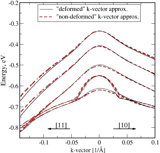
Transform crystal momentum because of strain

 strain-transforms-k-vectors = yes  ! 1D/2D/3D
                             = no   ! 1D/2D/3D

Ref. P. Enders et al., PRB, 51, 16695
"k.p theory of energy bands, wave functions, and optical selection rules in strained tetrahedral semiconductors"

The idea is the following:
If the elastic deformation is given by a relation r' = (1 + eps)r
then one has to perform a transformation k' = (1 - eps)k.
eps is du/dr and not just the symmetric part of it.
The flag is to decide if we want to do this transformation or not.

LOGICAL :: StrainTransforms_k_Vectors = .FALSE.  ! (default)
                                      = .TRUE.

Example by Michael Povolotskyi, University of Rome "Tor Vergata" (PhD Thesis):
The effect is small. And this is good, because if it were big that would mean that the method cannot be applied.
(5 nm 211 InAs/GaAs quantum well, 8x8 k.p calculation)

Broken gap type-II band alignment (for 8x8 k.p calculations)

broken-gap = no                 ! (default)
           = yes                !
           = full-band-density  ! FB-EFA (full-band envelope-function approach)

The following error for 8x8 k.p
Error update_kp: Cannot handle conduction band below valence band (E_cond_min < E_val_max).
can be avoided when using broken-gap = yes or broken-gap = full-band-density.
This error appears when the lowest conduction band edge value is lower than the highest valence band edge, i.e. a negative band gap is present.
In this case the code does not know how to distinguish between electron and hole states in an 8x8 k.p approach.
(Don't try to calculate the density when using broken-gap = yes.)
The density can be calculated using broken-gap = full-band-density.
This approach is termed FB-EFA (full-band envelope-function approach).
It is documented in detail in the following two papers:

• T. Andlauer, T. Zibold, P. Vogl
  Proc. SPIE 7222, 722211 (2009)
• Full-band envelope function approach for type-II broken-gap superlattices
  T. Andlauer, P. Vogl
  Physical Review B 80, 035304 (2009)

Piezo and pyroelectric charges at the boundaries

 piezo-charge-at-boundaries = no    ! 1D/2D/3D (default)
                            = yes   ! 1D/2D/3D
 pyro-charge-at-boundaries  = no    ! 1D/2D/3D (default)
                            = yes   ! 1D/2D/3D

To allow for piezo and pyroelectric charges at the boundaries. Usually nextnano³ sets the piezo and pyroelectric charges to zero at the boundaries of the device.

If one assumes that one only simulates a small part of the device (as is the case for most situations) one does not have an interface at the boundary (and therefore no charge).
If one wants to have an explicit interface at the boundary (because the device has a boundary there), one has to define a material-air interface in the input file. Alternatively one can use this option.
The corresponding charges can be looked up in the output file interface_densities1D.txt ($output-densities).
This option might be useful for wurtzite (pyroelectric charges) and strained zinc blende structures grown along other directions than [100] or [011] where there is a nonzero piezoelectric polarization P at the boundary. In vacuum P = 0. Therefore, there is div P nonequal to zero at the surface.

 

Set piezo and pyroelectric constants to zero (not implemented in latest version yet)

 piezo-constants-zero = no    ! 1D/2D/3D (default)
                      = yes   ! 1D/2D/3D
 pyro-constants-zero  = no    ! 1D/2D/3D (default)
                      = yes   ! 1D/2D/3D

To set the piezo any pyroelectric constants (piezo-electric-constants, pyro-polarization) from the database (database.in) or input file to zero. This option is useful to study the effects of piezo and pyroelectric charges in wurtzite independently. It is also useful for strained structures in order to understand the influence of strain much better.

Piezoelectric electric constant: Second order

 piezo-second-order         = no    ! 1D/2D/3D (default)
                            = yes   ! 1D/2D/3D

see e.g. G. Bester et al., PRL 96, 187602 (2006)

(preliminary feature, probably not tested and implemented sufficiently)

Discontinous quantum charge density at material interfaces in 1D and 2D

For the single-band Schrödinger equation in 1D and 2D, we need a parallel effective mass to calculate the quantum mechanical charge density. At material interfaces, this parallel effective mass is not continous (because the materials have different effective masses) which will lead to a discontinuity in the quantum mechanical charge density.
By default, we use an averaged parallel effective mass value which is weighted by the parallel effective masses at each grid point and the square of the wave function psi² at each grid point (FUNCTION get_mass_par_averaged). This will lead to a contious quantum mechanical charge density.
However, especially in 2D this could lead to an enormous increase in CPU time, especially if lots of eigenvalues are specified. Therefore the user can allow for discontinous parallel effective masses (and thus a discontinous quantum mechanical charge density) to speed up the calculations.

 discontinous-charge-density-1band = no    ! 1D/2D (default)
                                   = yes   ! 1D/2D

The figure on the left shows the quantum mechanical charge density of a 1D quantum well for the case of discontinous-charge-density-1band = yes.
The discontinuity in the parallel effective masses m(z) at material interfaces leads to a discontinuity in the quantum charge density at interfaces.

The right figure shows (for a different quantum well!) a comparison of the two approaches. The red line uses an averaged parallel effective m_o mass which leads to a continous quantum charge density (discontinous-charge-density-1band = no).
The x axis corresponds to the distance in nm, the y axis to the charge density in |e| * 1 * 10¹⁸ cm^-3.

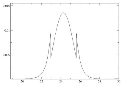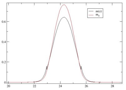
Superlattice

 superlattice-option             = whole                   ! (default)
                                 = 100-only                ! for dispersion along [100] direction, i.e. from Gamma to X
                                 = 010-only                ! for dispersion along [010] direction, i.e. from Gamma to X
                                 = 001-only                ! for dispersion along [001] direction, i.e. from Gamma to X
                                 = 110-only                ! for dispersion along [110] direction, i.e. from Gamma to K
                                 = 101-only                ! for dispersion along [101] direction, i.e. from Gamma to K
                                 = 001-only                ! for dispersion along [001] direction, i.e. from Gamma to K
                                 = 111-only                ! for dispersion along [111] direction, i.e. from Gamma to L
 Here one can specify if one wants to calculate the superlattice dispersion for the whole superlattice Brillouin zone,
  or along special directions in the superlattice Brillouin zone.
 Note that the directions refer to the simulation coordinate system and not to the crystal coordinate system.
  Internally, only positive K_SL values are calculated.

 superlattice-save-wavefunctions = yes                     ! (default)
                                 = no                      !
 no: Program will not save wave functions for K_SL vectors.
 Usually one is interested only in the eigenvalues and not so much in the wave functions itself.
 This option is necessary to avoid huge memory allocation, e.g. especially in 3D for option whole.

Exchange-Correlation (XC)

 exchange-correlation            = no               ! (default)
                                 = LDA              ! LDA   = local        density approximation
                                 = LSDA             ! LSDA = local spin density approximation
                                 = LDA-exchange     !             local        density approximation (only exchange,  for testing)
                                 = LSDA-exchange    !             local spin density approximation (only exchange,  for testing)
                                 = LDA-correlation  !             local        density approximation (only correlation, for testing)
                                 = LSDA-correlation !             local spin density approximation (only correlation, for testing)

Calculates exchange and correlation potentials as a functional of the density in LDA or LSDA.

Parameters for Ceperley-Alder model from J.P. Perdew and A. Zunger, Phys. Rev. B 23, 5048 (1981)
Depending on the type of polarization ([ unpolarized (LDA) , polarized (LSDA) ]), different sets of parameters have to be used.

        [ unpolarized , polarized ]
gamma = [  -0.1423d0  , -0.0843d0 ]
beta1 = [   1.0529d0  ,  1.3981d0 ]
beta2 = [   0.3334d0  ,  0.2611d0 ]
A     = [   0.0311d0  ,  0.0155d0 ]
B     = [  -0.048d0   , -0.0269d0 ]
C     = [   0.0020d0  ,  0.0007d0 ]
D     = [  -0.0116d0  , -0.0048d0 ]

Exciton

 coulomb-matrix-element                 = yes
                                        = no
 To output Coulomb energy (= Hartree energy) only (does not work yet).

 calculate-exciton                      = yes  ! 1D/3D
                                        = no   ! 1D/3D
 3D: To calculate exciton energy of electron and heavy hole state self-consistently (Hartree approximation only).
        It is also possible to calculate the exction energy of electron and light hole, or electron and split-off hole.
 

 exciton-iterations                     = 5    ! 3D for self-consistency loop (Hartree only)
 Note: For self-consistent Kohn-Sham eigenvalue problem, exiton-iterations must be set too a much higher value (!).
 There are two situations where exciton-iterations is used for self-consistent Kohn-Sham eigenvalue problem:
  - SUBROUTINE calc_exciton             (=> exciton-iterations =  50)
  - SUBROUTINE calc_many_body_state_LSD (=> exciton-iterations = 150)

 exciton-residual                       = 1d-5 ! 3D for self-consistency loop
 There are two further situations where exciton-residual is used, namely for self-consistent Kohn-Sham eigenvalue problem:
  - SUBROUTINE calc_exciton             (=> exciton-residual = 1d-5)
  - SUBROUTINE calc_many_body_state_LSD (=> exciton-residual = 1d-6)

 exciton-electron-state-number          = 1    ! 1D/3D electron ground state
                                        = 2    ! 1D/3D 2^nd electron state
                                        = ...
 exciton-hole-state-number              = 1    ! 1D/3D hole ground state
                                        = 2    ! 1D/3D 2^nd hole state
                                        = ...
 For example with these integer numbers it is possible to specify:
 - Calculate exciton energy of the electron ground state with the hole ground state.
 - Calculate exciton energy of the 2^nd electron state with the hole ground state.
 - Calculate exciton energy of the electron ground state with the 2^nd hole state.
 - Calculate exciton energy of the 2^nd electron state with the 2^nd hole state.

Note: The numbering of k.p states is twice as many as single-band because spin up and spin down states are included.
Example: The 1^st k.p hole state corresponds to the 1^st single-band holes state.
        The 3^rd k.p hole state corresponds to the 2^nd single-band holes state.
        The 5^rd k.p hole state corresponds to the 3^nd single-band holes state.


3D:
number-of-electron-states-for-exciton   = 3    ! 2D
number-of-hole-states-for-exciton       = 3    ! 2D

In 2D, these two specifiers specify the number of electron and hole states that are considered for the wave function expansion, i.e. 3 means 1 electron ground state and 2 excited electron states and similar for the holes.


2D:
exciton: X0
-----------
 number-of-electron-states-for-exciton  = 1    ! electron ground state
 number-of-hole-states-for-exciton      = 1    ! hole ground state

biexciton: XX0
--------------
 number-of-electron-states-for-exciton  = 2    ! 2 lowest electron states
 number-of-hole-states-for-exciton      = 2    ! 2 highest hole states

Not implemented yet:

charged exciton: X-
-------------------
 number-of-electron-states-for-exciton  = 2    ! 2 lowest electron states
 number-of-hole-states-for-exciton      = 1    ! hole ground state

charged exciton: X+
-------------------
 number-of-electron-states-for-exciton  = 1    ! electron ground state
 number-of-hole-states-for-exciton      = 2    ! 2 highest hole states

Note: The numbering of k.p states is twice as many as single-band because spin up and spin down states are included.
Example: The 1^st k.p hole state corresponds to the 1^st single-band holes state.
        The 3^rd k.p hole state corresponds to the 2^nd single-band holes state.
        The 5^rd k.p hole state corresponds to the 3^nd single-band holes state.
 

In 1D we currently have a routine that calculates the exciton correction in type-I quantum wells (single-band only, suited for electron and hole ground states only).
See tutorial "Exciton energy in quantum wells":
The 1D output can be found here: sg_1band1/exciton_energy1D.dat
It contains information on the exciton binding energy (in units of [meV] and [Rydberg]) and on the exciton Bohr radius (which is the variational parameter) in units of [nm].

To speed up the calculations, the user can provide an educated guess for the start value of the variational parameter lambda.
Both of the following inputs are optional;
 exciton-lambda             = 2.0d0   ! [nm] 1D only (optional)
 exciton-lambda-step-length = 0.05d0  ! [nm] 1D only (optional)
If they are not present, then internally calculated values are taken:
 ==> exciton-lambda             =  BohrRadius2DLimit
 ==> exciton-lambda-step-length = (BohrRadiusBulkExciton - BohrRadius2DLimit) / (lambda_steps - 1)

Note for 1D:
If 'debug-level > 0', then the code does not exit when the minimum of the exciton binding energy has been found.


In 3D we can calculate the exciton correction in quantum dots taking into account the Coulomb potential (Hartree approximation).
This works for single-band Schrödinger equation for both electrons and holes, as well as for 8x8 k.p for both electrons and holes. One can also treat the electrons within single-band and the holes within 6x6 k.p.

The following output files are provided:

Exciton ground state

    sg_1band1/exciton_energy3D_cb001_vb001.dat (At present, also for k.p calculations the output directory is the single-band directory.)
                                     vb001 (= heavy hole)
                                     vb002 (= light hole)
                                     vb003 (= split-off hole)

    E field [V/m],   E_ex [eV],      E_el - E_hl,    E_el0 - E_hl0,   Delta_Ex,       REAL(inter_matV(1))
    ...
    0.000000E+000    0.788262E+000   0.778266E+000   0.797671E+000    0.940847E-002   0.992412E+000

E field [V/m]:       Electric field value (not fully implemented and tested yet)
                     E field = voltage-offset / lever-arm-length
                     For details, see $output-1-band-schroedinger.
E_ex [eV]:           Energy of the exciton state
                     E_ex = E_el - E_hl - 0.5d0 * (mat_el - mat_hl)  (Eq. (6.37), p. 79 in diploma thesis of Matthias Sabathil)
                     matrix element mat_el = < psi_hl | V_psi_el | psi_hl >
                     matrix element mat_hl = < psi_el | V_psi_hl | psi_el >
E_el  - E_hl  [eV]:  Energy of the electron state minus the hole state
E_el0 - E_hl0 [eV]:  Transition energy of the original electron state minus the original hole state (without exciton correction), i.e.
                     energy difference between non-interacting electron and hole one-particle states.
Delta_Ex [eV]:       Energy difference due to exciton correction, i.e. between the energy difference of the eigenvalues of the
                     non-interacting electron and hole one-particle states (E_el0 - E_hl0) and the energy of the exciton state E_ex.
                     Delta_Ex = E_el0 - E_hl0 - E_ex  (Eq. (6.38), p. 79 in diploma thesis of Matthias Sabathil)
REAL(inter_matV(1)): single-band case: | SUM(psi_el * psi_hl) |2
                     k.p: optical matrix element


Biexciton ground state

    sg_1band1/biexciton_energy3D_cb001_vb001.dat (At present, also for k.p calculations the output directory is the single-band directory.)
                                       vb001 (= heavy hole)
                                       vb002 (= light hole)
                                       vb003 (= split-off hole)

    E field [V/m],   E_biex [eV],    E_el - E_hl,    E_el0 - E_hl0,   Delta_Ex,       REAL(inter_matV(1))
    ...
    0.000000E+000    0.254603E+001   0.128976E+001   0.135468E+001    0.163326E+000   0.000000E+000

E field [V/m]:       Electric field value (not fully implemented and tested yet)
                     E field = voltage-offset / lever-arm-length
                     For details, see $output-1-band-schroedinger.
E_biex [eV]:         Energy of the biexciton state
                     E_biex = 2 (E_el - E_hl) - 4 * 0.5d0 * (mat_el - mat_hl) - mat_elel - mat_hlhl (Eq. on p. 65 in PhD thesis of O. Stier, TU Berlin)
                     matrix element mat_el   =   < psi_hl | V_psi_el | psi_hl >
                     matrix element mat_hl   =   < psi_el | V_psi_hl | psi_el >
                     matrix element mat_elel =   < psi_el | V_psi_el | psi_el >
                     matrix element mat_hlhl = - < psi_hl | V_psi_hl | psi_hl >
E_el  - E_hl  [eV]:  Energy of the electron state minus the hole state
E_el0 - E_hl0 [eV]:  Transition energy of the original electron state minus the original hole state (without biexciton correction), i.e.
                     energy difference between non-interacting electron and hole one-particle states.
Delta_Ex [eV]:       Energy difference due to biexciton correction, i.e. between the energy difference of the eigenvalues of the
                     non-interacting electron and hole one-particle states 2*(E_el0 - E_hl0) and the energy of the biexciton state E_biex.
                     Delta_Ex = 2*(E_el0 - E_hl0) - E_biex
REAL(inter_matV(1)): single-band case: | SUM(psi_el * psi_hl) |2
                     k.p: optical matrix element


Note: There might be problems with the current nextnano³ implementation of the exciton routines for electrons at other valleys than Gamma (due to degeneracies, splitting of bands) or for the light holes (single-band approximation).

Tight-binding: Method and parameters

tight-binding-method = bulk-zincblende-sp3s*-nn     !     nn =        nearest-neighbor
                     = bulk-graphene-Saito-nn       !     nn =        nearest-neighbor
                     = bulk-graphene-Scholz-nn      !     nn =        nearest-neighbor
                     = bulk-graphene-Scholz-3rd-nn  ! 3rd-nn = third-nearest-neighbor
                     = bulk-graphene-Reich-3rd-nn   ! 3rd-nn = third-nearest-neighbor

The units are [eV]. 16 parameters are required for zinc blende materials.

tight-binding-parameters = -3.53284d0 ! Esa         (GaAs)
                            0.27772d0 ! Epa
                           -8.11499d0 ! Esc
                            4.57341d0 ! Epc
                           12.33930d0 ! Es_a
                            4.31241d0 ! Es_c
                           -6.87653d0 ! Vss
                            1.33572d0 ! Vxx
                            5.07596d0 ! Vxy
                            0d0       ! Vs_s_
                            2.85929d0 ! Vsa_pc
                           11.09774d0 ! Vsc_pa
                            6.31619d0 ! Vs_a_pc
                            5.02335d0 ! Vs_c_pa
                            0.32703d0 ! Delta_so_a
                            0.12000d0 ! Delta_so_c

Note: Special case for graphene (3 parameters only, nearest-neighbor tight-binding approximation):

 tight-binding-parameters =  0d0     ! [eV] E_2p: site energy of the 2p_z atomic orbital (orbital energy)
                            -3.013d0 ! [eV] gamma₀: C-C transfer energy (nearest-neighbor, nn)
                             0.129d0 ! []   s₀: denotes the overlap of the electronic wave function on adjacent sites (nn)

Note: Special case for graphene (7 parameters only, third-nearest-neighbor tight-binding approximation):

 tight-binding-parameters = -0.28d0  ! [eV] E_2p: site energy of the 2p_z atomic orbital (orbital energy)
                            -2.97d0  ! [eV] gamma₀: C-C transfer energy (nearest-neighbor, nn)
                             0.073d0 ! []   s₀: denotes the overlap of the electronic wave function on adjacent sites (nn)
                            -0.073d0 ! [eV] gamma₁: (2^nd-nn)
                             0.018d0 ! []   s₁:          (2^nd-nn)
                            -0.33d0  ! [eV] gamma₂: (3^rd-nn)
                             0.026d0 ! []   s₂:          (3^rd-nn)

Special option for third-nearest-neighbor tight-binding approximation in graphene:

tight-binding-calculate-parameter = no     ! (default) use 7 parameters (E_2p,gamma₀,gamma₁,gamma₂,s₀,s₁,s₂)
                                  = E2p    !             use 6 parameters (       gamma₀,gamma₁,gamma₂,s₀,s₁,s₂)
                                  = gamma1 !             use 6 parameters (E_2p,gamma₀,             gamma₂,s₀,s₁,s₂)
E_2p or gamma₁ can be calculated internally in order to force E(K) = 0 eV where K is the K point in the Brillouin zone. In that case, only 6 parameters are used (although 7 parameters have to be present in the input file). The parameter to be calculated is simply ignored inside the code.

Graphene potential fluctuation

graphene-potential-fluctuation = 0d0                   0.0001d0               4d0         ! [eV] [eV] [] (default)
                               = 0d0                   0.0001d0                           ! [eV] [eV]
                               = 0d0                                                      ! [eV] (default, i.e. "ideal" graphene layer)
                               = 0.100d0                                                  ! [eV]
                               = 0.100d0               0.001d0                3d0         ! [eV] [eV] [] These are useful values, especially the latter two for CPU efficiency.
                               = PotentialFluctuation  EnergyGridResolution  sigma_factor ! [eV] [eV] []

For Dirac point potential fluctuation see H. Xu et al,. APL 98, 133122 (2011).
We assume a Gaussian distribution of the potential fluctuation.
The 1^st value of these array entries corresponds to the fluctuation in potential energy of the Dirac point in units of [eV]. Useful values lie in the range from 0 eV to 0.200 eV.
The 2^nd value of these array entries (optional) corresponds to the energy grid resolution of the Gaussian integration in units of [eV].
The 3^rd value of these array entries (optional) is related to the integration range of the Gaussian integration in units of [].
The integration range is from [ - sigma_factor *  PotentialFluctuation , + sigma_factor *  PotentialFluctuation ] [eV].
Adjusting the 2^nd and 3^rd value has implications on CPU time. 3d0 is a very reasonable value for sigma_factor and also an energy grid resolution of 1 meV (0.001d0) is sufficient.

CBR method

 get-k-vector-dispersion-for-lead-modes = arccos ! (default)
                                        = use_ln !
                                        = acosIN ! use intrinisc arccosine function DACOS (only for testing)
 

In principle, all methods for arcos(x) = cos^-1(x) should be identical. (acosIN only for certain energy range where k is real.)

At present, it seems that use_ln works for electrons only.                 (for holes: 'mass' is negative)
                 It seems that arccos works for both, electrons and holes. (for holes: 'mass' is negative)

k = 1 / dx * cos^-1 ( ( E - E_l,m ) / 2 t - 1 )

For more details, see Matthias Sabathil's documentation of CBR_example, page 4 ("Lead modes").