nextnano³ - Tutorial

next generation 3D nano device simulator

1D Tutorial

Solution of the Poisson equation for different charge density profiles

Note: This tutorial's copyright is owned by Stefan Birner, www.nextnano.de.

Author: Stefan Birner
Please send comments to nextnano3 (-at-) wsi.tum.de.

If you want to obtain the input files that are used within this tutorial, please contact stefan.birner@nextnano.de.
1) -> 1D_Poisson_dipole.in
2) -> 1D_Poisson_linear.in
3) -> 1D_Poisson_delta.in
 

1) Dipole: Constant charge density profile of positive and negative charge

2) Linear charge density profile of positive and negative charge

3) Delta-function like charge density profile of positive and negative charges

1) Dipole: Constant charge density profile of positive and negative charge

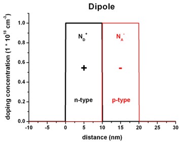
The following figures show a dipole charge density distribution where
- the left   region carries a constant positive  charge density (resulting from ionized donors     N_D⁺) and
- the right region carries a constant negative charge density (resulting from ionized acceptors N_A^-).

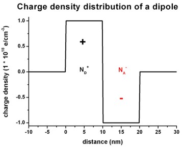
Left figure:  1Ddoping_concentration.dat
Right figure: densities1/density1Dspace_charge.dat

      

We have to solve the Poisson equation: d²phi / dx² = - rho / (epsilon epsilon₀)

The following figures shows the corresponding electric field distribution (left) and the electrostatic potential (right).

Left figure:  band_struc1/electric_field1D.dat
Right figure: band_struc1/potential1D.dat

      

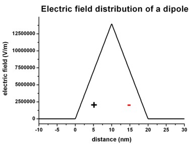
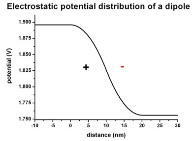
The electric field is given by E(x) = - dphi / dx and has a linear dependence (~ -x) because the electrostatic potential has a quadratic dependence (~ x²).

The maximum value of the electric field is given by:

E_max = rho / (epsilon epsilon₀) * x₀ = e * 1*10¹⁸ cm^-3 / ( 12.93 * 8.8542*10^-12 As/Vm ) * 10 nm =
        = 1.3995*10⁷ V/m = 139.95 kV/cm

where x₀ is the width of the positive (or negative) charge density region, and epsilon = 12.93 is the static dielectric constant of GaAs.

The drop of the electrostatic potential between 0 nm and 20 nm is simply given by the area that is below the graph of the electric field:

       Delta phi = 1/2 E_max * 20 nm = 139.95 meV

2) Linear charge density profile of positive and negative charge

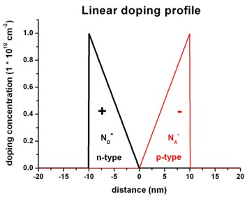
The following figures show a linearly varying charge density distribution where
- the left   region carries a linearly decreasing positive  charge density (resulting from ionized donors     N_D⁺) and
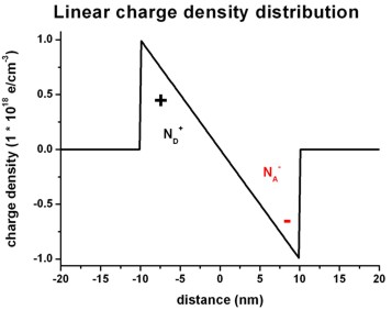
- the right region carries a linearly increasing  negative charge density (resulting from ionized acceptors N_A^-).

Left figure:  1Ddoping_concentration.dat
Right figure: densities1/density1Dspace_charge.dat

        

The following figures shows the corresponding electric field distribution (left) and the electrostatic potential (right).

Left figure:  band_struc1/electric_field1D.dat
Right figure: band_struc1/potential1D.dat

   

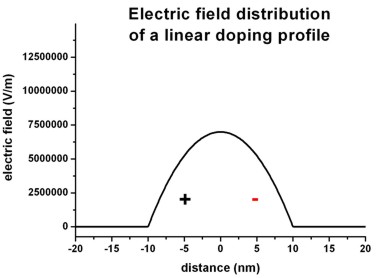
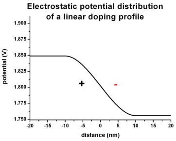
The electric field shows a quadratic dependence  (~ -x²) whereas the electrostatic potential shows a cubic dependence (~ x³).

3) Delta-function like charge density profile of positive and negative charges

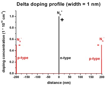
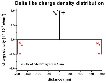
The following figures show a delta-function like charge density distribution where
- in the middle       of the structure there is a constant positive  charge density   of width 1 nm         (resulting from ionized donors     N_D⁺) and
- at the boundaries of the structure there are constant negative charge densities of width 1 nm each (resulting from ionized acceptors N_A^-).

Left figure:  1Ddoping_concentration.dat
Right figure: densities1/density1Dspace_charge.dat

        

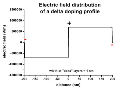
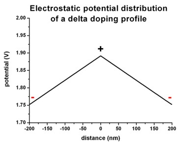
The following figures shows the corresponding electric field distribution (left) and the electrostatic potential (right).

Left figure:  band_struc1/electric_field1D.dat
Right figure: band_struc1/potential1D.dat

   

• Please help us to improve our tutorial. Send comments to nextnano3 (-at-) wsi.tum.de.