doping-function
Doping profiles
Doping profiles can be specified by the product of n functions. n is the dimension of the simulation,
i.e. n = 1, 2 or 3. Each function depends only on
one coordinate.
The doping profile is independent of the regions specified before. The
function is applied to the region given by the specifier only-region.
The doping concentration is at the position specified by the specifier
position.
The function is normalized such that the result is doping concentration at
position position.
The impurity number specifies the kind of impurities used in the profile.
Note: Can be used with a doping
concentration sweep where the doping-concentration is varied
stepwise.
!------------------------------------------------------------------!
$doping-function
optional   !
 doping-function-number
integer
required   !
 impurity-number
integer
required   !
 base-function-1
character
optional   !
 base-function-2
character
optional   !
 base-function-3
character
optional   !
 apply-function-1-along-dir
integer_array   optional   !
 apply-function-2-along-dir
integer_array   optional   !
 apply-function-3-along-dir
integer_array   optional   !
 doping-concentration
double
required
!
 position
double_array    optional
!
 parameters-base-function-1
double_array
optional   !
 parameters-base-function-2
double_array
optional   !
 parameters-base-function-3
double_array
optional   !
 exclude-materials
integer_array   optional   !
 only-region
double_array
optional   !


!

 doping-profile-defined-by-function
character
optional   !
new
!

 read-in-doping-file
character
optional   !

 doping-filename
character
optional   !
!

 doping-sweep-active
character
optional   !
 doping-sweep-step-size
double
optional
!
 doping-sweep-number-of-steps
integer
optional
!
$end_doping-function
optional   !
!------------------------------------------------------------------!
Example
Constant doping profile
 $doping-function


  doping-function-number = 1

  impurity-number        =
1
!
properties of this impurity type have to be here:
$impurity-parameters
  doping-concentration   = 0.5d0
! 0.5 * 10^18 cm^-3

  only-region
= 10.0d0 160.0d0


 $end_doping-function
Note: Can be used with a doping
concentration sweep where the doping-concentration is varied
stepwise.
doping-function-number = 1


= 2


= ...
An integer number. At the very end, the doping function numbers must be given in
a way, that a dense ascending series starting at 1
can be formed.
impurity-number = 1


 = 2


 = ...
An integer number. Properties of this impurity number have to be specified
later.
This is a reference to an impurity and its parameters which will be specified by
$impurity-parameters.
More complicated doping profiles
You can use different base functions along each simulation direction
to define more complicated doping profiles.
base-function-1 = string-1
base-function-2 = string-2
base-function-3 = string-3
a valid base function name
string-i can be one of the one-dimensional functions:
constant,
linear,
gauss-1d,
step-1d,
well-1d
The final doping profile will result from a product of these functions.
parameters-base-function-1 = double1 ....
parameters-base-function-2 = double1 ....
parameters-base-function-3 = double1 ....
function parameters
Parameters for the selected base functions. Dependent on the base function
chosen, the following is expected:
Constant base function: Constant doping profile
base-function-1 = constant
No further function parameters required in 1D simulations.
Note: Can be used with a doping
concentration sweep where the doping-concentration is varied
stepwise.
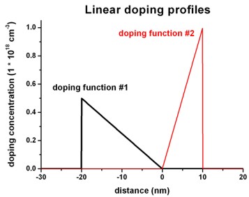
Linear base function: Linear doping profile
base-function-1            =
linear
The example shows which additional parameters are necessary.
Example:
$doping-function


 doping-function-number     =
1
!
doping function #1
 impurity-number
= 1
!
 doping-concentration       =
0.5d0
! 0.5 * 1.0 * 10^18 cm^-3 = 0.5 * 10^18 cm^-3

 position
= -20d0
! -20 nm
 only-region
= -20d0 0d0
! -20 nm to 0 nm
 base-function-1
= linear
!
 apply-function-1-along-dir = 0 0 1

!
 parameters-base-function-1 = -20d0 0d0
0.5d0 0.0d0 ! (1) zmin = -20 nm
(2) zmax = 0 nm


! (3) 0.5 * 10^18 cm^-3  (4)
0.0 * 10^18 cm^-3


 doping-function-number
= 2
!
 impurity-number
= 2
!
 doping-concentration       =
1d0
! 1.0 * 10^18 cm^-3

 position
= 10d0
!
 only-region
= 0d0 10d0
!
 base-function-1
= linear
!
 apply-function-1-along-dir = 0 0 1

!
 parameters-base-function-1 = 0d0 10d0
0.0d0 1.0d0 ! (1) zmin = 0 nm
(2) zmax = 10 nm


! (3) 0.0 * 10^18 cm^-3   (4)
1.0 * 10^18 cm^-3


$end_doping-function
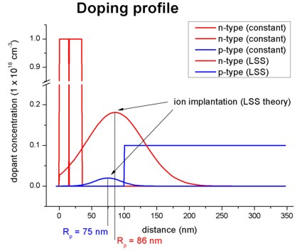
LSS theory (Lindhard, Scharff, Schiott theory) -
Gaussian distribution of ion implantation impurity profile
base-function-1            = gauss-1d
!
LSS theory
parameters-base-function-1 = center-coordinate
gauss-width         minimum-value  maximum-value

center-coordinate
is the position of the Gauss center along the
relevant direction i in units of
[nm].
gauss-width [nm]).
For the meaning of gauss-width
have a look at the
10 DM
banknote of the German "Deutsche Mark" or any mathematical textbook.
minimum-value minimum value of doping concentration
in units of 1018 [cm-3]
maximum-value maximum value of doping concentration
in units of 1018 [cm-3]
Within LSS theory the specifiers correspond to the following notations:
base-function-1            = gauss-1d
!
LSS theory
parameters-base-function-1 = projected-range
projected-straggle
minimum-value  maximum-value

apply-function-1-along-dir = 0 0 1
!
along z direction
doping-concentration       =
implanted-dose / ( SQRT(2*pi) * projected-straggle )
!
concentration at reference position
(see below)
position                   =
projected-range  !
projected-range [nm], i.e. the depth where most ions stop.
projected-straggle Delta Rp
(ion straggle) in units of [nm], i.e. the statistical fluctuation
of Rp.
implanted-dose
phi in units of [1/cm^2] (dose of the implant), typical ranges are
from 1d11 to
1d16.
$output-material
and the specifier doping-concentration.
For further details see for example:
"Very brief
Introduction to Ion Implantation for Semiconductor Manufacturing" by Gerhard
Spitzlsperger
User-defined doping function
Using the specifier
doping-profile-defined-by-function, one can define an arbitrary function
n(x,y,z) for the doping profile.
The value of this function is finally multiplied by the value specified in
doping-concentration. Obviously, one can also set
doping-concentration = 1d0.
The variables x, y, z refer to the grid point coordinates of the simulation area
in units of [nm].
Example: The red Gaussian shaped curve in
the above figure can also be achieved by defining the Gaussian function
directly:
$doping-function

 ...

   %mu      =
86
!    mu
of Gaussian distribution (DisplayUnit:nm)
%sigma =
44
! sigma of Gaussian distribution (DisplayUnit:nm)
%max_dop =
0.181337400182469
! maximum doping concentration at center of Gaussian distribution
(DisplayUnit:1e18cm^-3)


 doping-function-number             =
4
!
doping function #4
 impurity-number
= 2
!

 doping-concentration
= %max_dop        ! 1
* 10^18 cm^-3

 doping-profile-defined-by-function = " exp(-
(z-%mu)^2 / (2*%sigma^2)
) "  ! n(x,y,z) = ...
= no !
The following operators and functions are supported:
+ , - ,
	* , / , ^

	abs , exp , sqrt
	, log , log10
	, sin , cos
	, tan , sinh ,
	cosh , tanh , asin
	, acos , atan
Predefined doping functions
base-function-1 = step-1d
parameters-base-function-1 = para(1) = center, para(2) = width, para(3) =
leftval, para(4) = rightval
base-function-1 = well-1d
parameters-base-function-1 = para(1) = center, para(2) = width, para(3) =
leftval, para(4) = rightval
para(5) = center, para(6) = width, para(7) = leftval, para(8) = rightval
First 4 parameters for left step, second 4 parameters for right step.
This is a well with double gauss walls. The walls are centered at parameter center
and the slope of the walls is given by width.
apply-function-1-along-dir = i j k
apply-function-2-along-dir = i j k
apply-function-3-along-dir = i j k
Variation of function-i is along the specified direction (0 0 1
or
0 1 0 or 1 0 0).
doping-concentration = double
concentration at reference position (see below).
A doping concentration at the position specified by the next specifier
(position). The function defined above is normalized such that the result is
doping concentration at position position.
Example:
We take a constant doping with a
concentration 8.0*1018
cm-3.
1D simulation: 8.0d0 * 1018/cm3.
doping-concentration =
  8.0d0
2D simulation: 8.0d0 * 1018/cm3.
   doping-concentration =
  8.0d0
3D simulation: 8.0d0 * 1018/cm3
doping-concentration =
8.0d0
So we take the value to be
8.0d0 because we assume a 3D
doping although we do a 1D or 2D simulation.
Thus it would be wrong to take
- 2.0 *106 cm-1
in the 1D case (cubic root)
- 4.0 *1012 cm-2
in the 2D case (squared cubic root)
position = coord1 ...
Doping concentration refers to that position.
The coordinates of a position which is used to fix normalization of the doping
function profile. Can be omitted only for constant doping.
exclude-materials = num1 ...
To keep certain materials free from doping (e.g. air).
A list of defined material numbers which should not be doped.
only-region = coord1 ...
Apply doping function only to this region (coordinates of a cube,
rectangle, line).
Restrict doping to this region only. The region is either a cube, rectangle or
a line. The coordinates given specify the extension of the region as usual.
Note: See comments on how to specify correct interfaces further below.
Example (2D):
$doping-function
!


!

 doping-function-number = 1
!

 impurity-number        =
1
!
properties of this impurity type have to be specified by
$impurity-parameters

 doping-concentration   = 10d0
!
10 * 1018/cm3.
 only-region
= 0.0d0 50.0d0 30.0d0 60.0d0 !
xmin xmax  ymin ymax


!

$end_doping-function
!
Note: It you want to generate a very "accurate" doping
profile, then you should apply the doping between interfaces. Interfaces
are set if the material number is different.
Example: You want to specify a doping
between 35.0 and 35.3 nm. Then you should consider to define a separate region,
a separate cluster and a separate material for this 0.3 nm region.
Accurate doping profile:
   35.0     35.15    35.3
! [nm]
     x        x
x        x
!
physical grid points
     |
|
!
    o|o       o
o|o       o
!
.
.       .
.             !
material grid points (material parameters)
----- _________________ ------------------!
    0|1       1       1|0
!
Not so accurate doping profile:
   35.0     35.15    35.3
! [nm]
     x        x
x        x
!
physical grid points
     |
! 35.3 nm
o|o o
o o
!
'multiple grid point' grid points (including multiple points)
.
.       .
.             !
material grid points (material parameters)
----- ____________________ ---------------!
    0|1       1       0.5
! (an average)
Another not so accurate doping profile:
   35.0     35.15    35.3
! [nm]
     x        x
x        x
!
physical grid points
!
     o        o
o        o
!
.
.       .
.             !
material grid points (material parameters)
-- _______________________ ---------------!
0.5 1 0.5 !
Obviously all three cases can produce different results.
Example (3D):
The following figure shows a 3D doping profile that is defined inside a 20 nm
x 20 nm x 50 nm cube where the 50 nm are the z direction. The doping profile is
homogeneous with respect to the (x,y) plane, it only varies along the z
direction.
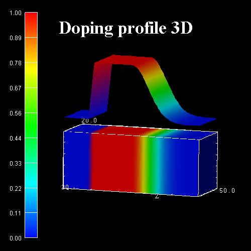
The doping profile is constant between z
= 10 nm and z = 25 nm with a concentration of 1 x 1018 cm-3.
It has Gaussian shape from z = 25 nm to z = 45 nm. It is
zero between z = 0 nm and z = 10 nm, as well as
between z = 45 nm and z = 50 nm.
 $doping-function


  !-------------------------------------

  ! constant doping of 1 * 10^18 cm^-3.

  !-------------------------------------

  doping-function-number     = 1
!
first doping funtion
  impurity-number
= 1
!

  doping-concentration       =
1.0d0
! 1.0d0 => 1.0 * 10^18 / cm^3

  only-region
= 0d0 20d0  0d0 20d0  10.0d0 25.0d0 !
xmin xmax  ymin ymax  zmin zmax


!--------------------------------------------------------------------------

  ! Gaussian shaped doping along z direction, constant doping in (x,y)
plane


!--------------------------------------------------------------------------


  doping-function-number     = 2
!
  impurity-number
= 1
 !

  only-region
= 0d0 20d0  0d0 20d0  25.0d0 45.0d0 !
xmin xmax  ymin ymax  zmin zmax


  base-function-1
= constant
!

  base-function-2
= constant
!

  base-function-3
= gauss-1d
!

  apply-function-1-along-dir = 1 0 0
!
  apply-function-2-along-dir = 0 1 0
!
  apply-function-3-along-dir = 0 0 1
!
  doping-concentration       =
1d0
! 1.0d0 => 1.0 * 10^18 / cm^3

  position
= 10d0 10d0 25d0
 !
  parameters-base-function-1 = 0d0 100d0

  parameters-base-function-2 = 0d0 100d0

  parameters-base-function-3 = 25d0 6d0  0d0
1.0d0
! center-coordinate  gauss-width  minimum-value  maximum-value


 $end_doping-function
If you want to obtain the input file that was used to obtain this 3D doping
profile plot (constant + Gaussian shape), please submit a support ticket.
-> 3Ddoping_profile.in
Reading in doping profiles from a file
read-in-doping-file = yes/no

-
flag for reading in doping profile from a file
-
valid for n-type and p-type doping
-
valid for arbitrary doping-function-number
- can be combined with explicitly specifying doping profile by input file
and by reading in doping profile from several files
- all doping functions will be added to the previously
specified values (like superpositions)
Restrictions:
- The value of this profile is finally multiplied by
doping-concentration. Obviously, one can also set
doping-concentration = 1d0.
- You can specify a region (only-region) for which the
doping file applies to, the outer region will not contribute.
doping-filename = doping_input.dat
                =
doping/doping_input.dat
doping filename to be read in (e.g. experimental values). The string can
include a folder name.
The ASCII file must contain 2 (1D), 3 (2D) or 4 (3D) columns in each line:
1D:
x coordinate [nm]
doping concentration [1*1018 cm-3]

...
...
2D:
x coordinate [nm]    y coordinate [nm]                       doping concentration [1*1018 cm-3]

...
...
...
3D:
x coordinate [nm]    y coordinate [nm]   z coordinate
[nm]
doping concentration [1*1018 cm-3]

...
...
...
...
The first line of this ASCII file can contain an optional header line with
column descriptors.
If you want to obtain an input file that shows how to import a doping profile
from a file
(1D_read_in_potential_and_doping_profiles.in,
2D_read_in_potential_and_doping_profiles.in,
3D_read_in_potential_and_doping_profiles.in),
please submit a support ticket.
It is possible to sweep over the doping concentration, i.e. to vary the
doping concentration stepwise.
In each doping sweep step, the specifier doping-concentration is
increased by doping-sweep-step-size in units of [1*1018 cm-3].
The output is labelled by ..._ind000.dat, ..._ind001.dat,
... for each doping sweep step.
 doping-sweep-active           =
yes       !
to
switch on doping sweep
= no !
 doping-sweep-step-size        =
0.2d0
!
increase doping concentration in each step by ... in units of
[1*1018 cm-3]


!
(This value can also be negative.)
 doping-sweep-number-of-steps  = 5
!
Restrictions:
- Voltage sweeps ($voltage-sweep)
and other sweeps cannot be combined with doping sweeps at present.
- Only one doping sweep is allowed at present.
|