|
| |
nextnano3 - Tutorial
next generation 3D nano device simulator
2D Tutorial
Vertically coupled quantum wires in a longitudinal magnetic field
Author:
Stefan Birner
If you want to obtain the input files that are used within this tutorial, please
check if you can find them in the installation directory.
If you cannot find them, please submit a
Support Ticket.
 -> 1DAlGaAs_GaAs_DQW.in

 -> 1DGaAs_ParabolicQW_10meV.in

 -> 2DGaAs_CoupledQWRs_parabolic_10meV_APL2007.in
Vertically coupled quantum wires in a longitudinal magnetic field
In this tutorial we study the electron energy levels of two coupled quantum
wires as a function of a longitudinal (i.e. perpendicular) magnetic field.
This input file aims to reproduce Fig. 2 of
Vertically coupled quantum wires in a
longitudinal magnetic field
L.G. Mourokh, A.Y. Smirnov, S.F. Fischer
Applied Physics Letters 90, 132108 (2007).
Thus the following description is based on the explanations made therein.
The idea is to model experimental results which are shown in Fig. 8 (b) of this
paper:
Tunnel-coupled one-dimensional electron systems
with large subband separations
S.F. Fischer, G. Apetrii, U. Kunze, D. Schuh, G.
Abstreiter
Physical Review B 74, 115324 (2006)
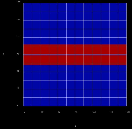
The following figure shows the layout of the structure in the (y,z) plane.
The blue regions are the barrier materials (Al0.32Ga0.68As)
and
the red regions are 14.5 nm GaAs quantum wells
that are separated by a 1 nm thin Al0.32Ga0.68As
tunnel barrier.
1D simulations
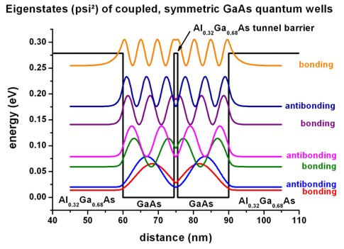
The following figure shows the confined eigenstates Ez of the
coupled, symmetric QW system (1D simulation along the z direction).
Note that the states have bonding and
antibonding character.
-> 1DAlGaAs_GaAs_DQW.in
The following material parameters were used:
- conduction band offset GaAs/Al0.32Ga0.68As:
CBO = 0.27882 eV
- electron effective mass GaAs:
me = 0.067 m0
-
The ground state (bonding state) has the
energy Ez,1 = 13.86 meV,
the antibonding state has the energy
Ez,2 = 19.78 meV,
thus the bonding-antibonding level separation is DeltaSAS = 5.92 meV.
To model quantum wires, instead of quantum wells, we follow the methodology
of the above cited paper and apply a harmonic oscillator potential in the
quantum well plane.
We construct such a potential by surrounding GaAs with an InxGa1-xAs
alloy that has a parabolic alloy profile in the y direction.
(Our "InAs" has the same material parameters than GaAs apart from the conduction
band edge energy which is used to model the parabolic confinement.)
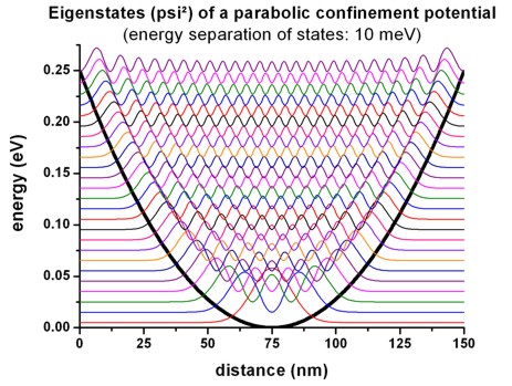
We illustrate this by a 1D simulation along the y direction: This
figure shows the eigenstates of the parabolic confinement potential.
The harmonic oscillator potential was chosen such that the energy separation of
the eigenstates is 10 meV, consequently the ground state is at 5 meV.
-> 1DGaAs_ParabolicQW_10meV.in
- 2D parabolic confinement with hbarw0 = 10 meV
Making use of the equation
- 1/2 ) hbarw0
where n = 1, 2, 3, ... and w0 = (C/m*)1/2
(m* = effective mass, C = constant which is related to the parabolic potential
V(y) = 1/2 K y2 )
one can calculate hbarw0:
- 0 eV = 10.06 meV
- Ey,1 = 10.05 meV
- Ey,2 = 10.05 meV
- Ey,3 = 10.06 meV
   ...

             Ey,1 =
	0.00503 eV

           Ey,2 =
	0.01508 eV

           Ey,3 =
	0.02513 eV

           Ey,4 =
	0.03519 eV
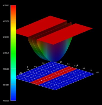
The following figure shows the conduction band edge profile of the two
coupled quantum wires. The confinement is as follows:
- along the y direction: parabolic confinement
- along the z direction: AlGaAs / GaAs / AlGaAs / GaAs / AlGaAs
heterostructure confinement
Along the x direction (perpendicular to the simulation plane), we will apply a
magnetic field to study the energy spectrum of the coupled quantum wires as a
function of longitudinal magnetic field.
-> 2DGaAs_CoupledQWRs_parabolic_10meV_APL2007.in
Magnetic field
- The magnetic field is oriented along the x direction, i.e. it is
perpendicular to the simulation plane which is oriented in the (y,z) plane.
We calculate the eigenstates for different magnetic field strengths (0
T, 0.5 T, 1.0 T,
..., 16 T), i.e. we make use of the magnetic field sweep.
  $magnetic-field
   magnetic-field-on
  = yes
   magnetic-field-strength
  = 0.0d0   !
1 Tesla = 1 Vs/m2
   magnetic-field-direction
  = 1 0 0   !
   magnetic-field-sweep-active
  = yes     !
   magnetic-field-sweep-step-size
  = 0.50d0  !
   magnetic-field-sweep-number-of-steps =
  32
  !
$end_magnetic-field
- A useful quantitiy is the magnetic length (or Landau magnetic length)
which is defined as:
lB = [hbar /
(me* wc)]1/2
= [hbar / (|e| B)]1/2
It is independent of the mass of the particle and depends only on the magnetic
field strength:
- 1 T: 25.6556 nm
- 2 T:
18.1413 nm
- 3 T: 14.8123 nm
- ...
- 20 T: 5.7368 nm
- The electron effective mass in GaAs is me* = 0.067 m0.
Another useful quantity is the cyclotron frequency:
wc
= |e| B / me*
Thus for the electrons in GaAs, it holds for the different magnetic field
strengths:
- 1 T: hbarwc = 1.7279 meV
- 2 T: hbarwc = 3.4558 meV
- 3 T: hbarwc = 5.1836 meV
-
- 20 T: hbarwc = 34.5575 meV
- The one-dimensional parabolic confinement (conduction band edge
confinement) was chosen so that the electron ground state has the energy of E1 = hbarw0
= 5 meV in the 1D simulation.
In the 2D simulation, the ground state has the energy: E1 = 18.64 meV (without magnetic field)
which corresponds approximately to
E1 ~= Ey,1 +
Ez,1 = 5.03 eV +
13.86 meV = 18.89 meV. (In 2D, we
use a different grid resolution compared to 1D simulations.)
Magnetic field
- The following figure shows the calculated energy spectrum, i.e. the eigenstates as a function of magnetic field magnitude:
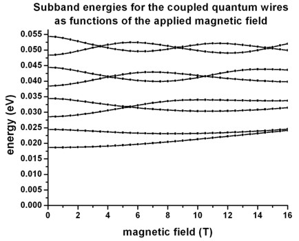
The figure is in excellent agreement with Fig. 2 of the above cited paper and
reproduces Fig. 8 (b) of the experimental paper very well.
For the physical significance of such a spectrum, we refer to the discussion
in the above cited papers.
- Note that each of the electron states is two-fold spin-degenerate. A magnetic field lifts this
degeneracy (Zeeman splitting). However, this effect is not taking into account
in this tutorial.
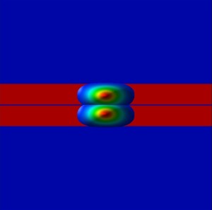
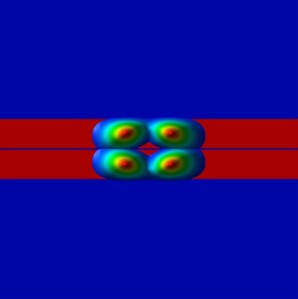
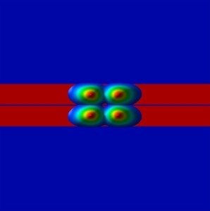
- The following figures show wave functions (psi2) of the lowest four eigenstates
- at zero magnetic field
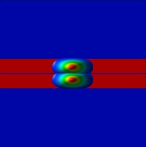

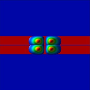
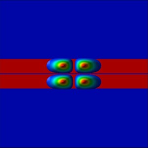
- at 5.5 T (where E3 and E4 have similar
energies)

|