|
| |
==> Our new software
nextnano.NEGF
has a different website: ==>
www.nextnano.com/nextnano.NEGF/
Quantum transport based on the Nonequilibrium Green's functions (NEGF)
method
The method of calculating the carrier transport is defined as "fully
self-consistent nonequilibrium Green's function (NEGF) approach for vertical
quantum transport in open quantum devices with contacts".
It is suited for calculating quantum transport and gain in quantum cascade
lasers.
This part of the
nextnano³ code is based on the original code of
Tillmann Kubis which
is described in these publications:
-
Quantum
transport in semiconductor nanostructures
T. C. Kubis
Selected Topics of Semiconductor Physics and Technology (G. Abstreiter,
M.-C. Amann, M. Stutzmann, and P. Vogl, eds.), vol. 114
Verein zur Förderung des Walter Schottky Instituts der Technischen
Universität München e.V., München (2009)
-
Modeling
techniques for quantum cascade lasers
C. Jirauschek, T. Kubis
Applied Physics Reviews 1, 011307 (2014)
-
Theory of nonequilibrium quantum transport and energy dissipation in
terahertz quantum cascade lasers
T. Kubis, C. Yeh, P. Vogl, A. Benz, G. Fasching, C. Deutsch
Physical Review B 79, 195323 (2009)
-
Self-consistent quantum transport theory: Applications and assessment of
approximate models
T. Kubis, P. Vogl
Journal of Computational Electronics
6,183 (2006)
There are several possibilities:
- to include several scattering mechanisms (e.g. inelastic scattering,
elastic scattering)
- no scattering at all ("ballistic transport")
The electrons are described within a one-band model with a variable effective
mass, i.e. a spatially dependent (= material dependent) effective electron mass
me(z). Alternatively, it is possible to use an energy dependent
effective mass (nonparabolicity). This nonparabolicity parameters are grid point
dependent. The static and optical dielectric constants
are also grid point dependent, i.e. material dependent.
This method is well suited to study resonant tunneling diodes and quantum
cascade lasers.
Restrictions for green:
- homogeneous grid
- not too much grid points (~50-100)
- for nextnano³: quantum cluster must extend over the whole device
- for nextnano³: two contacts at the boundaries having 2 grid points at the left and 2
grid points at the right contact,
material at the contacts should be the same as the semiconductor material
For an example of the Green's function functionality, have a look at the
RTD tutorial.
Global parameters for Green's function code
!--------------------------------------------------------------!

$global-parameters-NEGF
optional  !

 grid_points_in_z
integer
required  !

 grid_points_in_Ez
integer
optional  !

 grid_points_in_E
integer
optional  !

 contact_points
integer
optional  !

 non_diagonal_range
double
optional  ! [nm]

 max_energy_factor
double
optional  !

 Ez_grid_power
double
optional  !

 E_grid_power
double
optional  !

 grid_exponent
double
optional  !


 zero-drift-vector-in-contacts
character
optional  !

 use-maximum-drift-vector
character
optional  !

 drift-vector-maximum
double
optional  ! [nm-1]

 off_drift
double
optional  !


!

 fix-electric-field-at-contact
character
optional  !

 electric-field-at-contact
double
optional  ! [V/m]


!

 rescaling_green
character    optional
!
test!
!

 grid_limit
double
optional  !

 Poisson-damping-threshold
double
optional  !

 scatter_limit
double
optional  !

 limit-for-density-convergence
 double
optional  !

 grid_critical
double
optional  !


!

 gain
character    optional
!

 gain-output-every-nth-iteration
integer
 optional  !

 gain-integrate-device-from-to
double_array
optional  ! [nm]

 min_photon
double
 optional  ! [eV]

 max_photon
double
optional  ! [eV]

 photon_number
integer
 optional  !


!

 first-order-Born-approximation         character    optional
!


!

 solve-Poisson-equation
character    optional
!

 Poisson-Newton-method
character    optional
!

 Schroedinger-Poisson-Predictor
character
 optional  !

 Schroedinger-Poisson-Predictor-lambda  double
 optional  !

 built-in-potential
                    double
optional  !

 calculate-transmission
character    optional
!

 output-correlation-functions
character    optional
!

 output-quasi-Fermi-level
character    optional
!

 output-k-resolved
character    optional
!


!

 read-inputfile-during-calculation
character    optional
!

 include-original-NEGF-output
character    optional
!


!

 get-cb-from-nextnano
character    optional
!

 get-potential-from-nextnano            character    optional
!

 get-cb-masses-from-nextnano
character    optional
!

 get-nonparabolicity-from-nextnano
character
 optional  !

 get-dielectric-from-nextnano
character    optional
!

 get-alloy-from-nextnano

character    optional
!

 get-doping-from-nextnano
character    optional
!


!

 directory-NEGF

    character    optional
!

 directory-contact

    character    optional
!

 directory-scattering-rates
character    optional
!

 directory-test-debug

character    optional  !

 directory-stop

character    optional  !

 save-every-nth-iteration

integer      optional  !

 number-of-MKL-threads                  integer
 optional  !

 MKL-set-dynamic
        character    optional
!


!

$end_global-parameters-NEGF
 optional  !

!--------------------------------------------------------------!
!----------------------------------------------------------!

$global-parameters-NEGF

!
 grid_points_in_z
= 40
!
number of grid points in real space along z direction
! - 1 = grid_points_in_z
grid_points_in_E
= 110
! E = total energy
 grid_points_in_Ez
= 110
! Ez = E - hbar2 *
k||2 / [2m(1,E)]
! 1 = 1st grid point, the mass
m could depend on energy
E


!
The in-plane momentum k|| is represented as an energy Ez.
!non_diagonal_range
= 1d0
! [nm]
 non_diagonal_range
= 3d0
! [nm]
!non_diagonal_range
= 8d0
! [nm] 8d0 The default value
is 6d0.
!
!
! non_diagonal_range is converted to the
corresponding number of grid points that are involved. This depends on the grid
spacing, obviously.
! Nr_dself = nondiagonal_range / (It
always holds: Nr_dself >= 1)
! Nr_dself = (z,z') bands of the
self-energies, (i.e. 0 = diagonal, 1 = tridiagonal ... Nr_dself <= grid_points_in_z)
! number of nonvanishing diagonals in the inverse retarded Green's
function = 2*Nr_dself + 1
! If the distance between z3 and z4 (nonlocal
range) is longer than non_diagonal_range, the self-energies for the
LO and TO phonon scattering
! and impurity scattering (described by eq. (3.5.6) and eq. (3.5.52) of
T. Kubis' PhD thesis) are set to zero.
!
!

 contact_points
= 27                    !
27 27 contact grid points for the
right lead, i.e. in total 54 lead grid points (default =
5).
!
contact_points must be larger than (non_diagonal_range
/ grid_spacing) + 1 = Nr_dself + 1.
!-----------------------------------------------------------
!
!-----------------------------------------------------------
fix-electric-field-at-contact =
yes !
!
electric-field-at-contact.
!
The voltage drop will be achieved with drift vector.
=
no
! Determine the
electric field at the contacts self-consistently.
electric-field-at-contact
=
0d0 !
[V/m]
0d0
= flat band, i.e. constant electrostatic potential at
the left boundary = zero electric field)
!
electric-field-at-contact
is only relevant if fix-electric-field-at-contact =
yes.
!
electric-field-at-contact
applies to left contact. The right contact is identical unless the dielectric
constants of the left and right contacts are different.
!-----------------------------------------------------------
zero-drift-vector-in-contacts
= yes
!
semiconductor drift vector in the contacts, yes =
equilibrium contacts
=
no
!
no =
use-maximum-drift-vector
= no
!
zero-drift-vector-in-contacts = no, then
use-maximum-drift-vector can be yes.
! In this case, the drift vector is set to its maximum.
! zero-drift-vector-in-contacts = yes, then
use-maximum-drift-vector is not used at all.
! fix-electric-field-at-contact = no
and entropicL = .FALSE..
!
drift-vector-maximum
= 5.0d0
! [nm-1]
off_drift
= 0d0
! should be zero
!
!Ez_grid_power
= 2d0
! n, i.e. xn
- if present, static Ez grid
! Ez grid: (grid point no.)^n + offset
! if not present, a self-consistent multigrid for Ez is used
!E_grid_power
= 1d0
! Ez_grid_power, but here for E grid
grid_exponent
= -0.3d0 ! -0.3d0 ! (/=0, a negative is
preferred), controls the dynamical Ez grid, if approximately=0, then
linear grid
! 0.01d0) gives an
almost linear grid
max_energy_factor
= 9.90d0
! []
! max_energy_factor = - ln fmin
! fmin is the state occupancy which is
typically considered to be empty,
! fmin ~ 5 * 10^-5 ==> max_energy_factor ~ 9.90,
! default: 0.9d0
!
!
max_energy_factor * kBT is smaller than '2
ELO' than the energy value of two LO phonon energies ELO
is taken instead.
!
grid_limit
= 0.05d0
! [] -0.05d0)
! E
and Ez will not be changed any more.
Poisson-damping-threshold
= 1d0
! 1d0
! This value determines the criteria which of the Poisson-damping
parameters is used. It is related to convergence of the density.
scatter_limit
= 1d0
! 1d0)
limit-for-density-convergence
= 5d-5 !
[]
5d-5
grid_critical
= 1d-10
! used for determining resonances in the total device (default:
1d-10)
!
find_hot_spots that is used for the self-adapting energy
grid Ez.
!
! Ez.)
!
!
!
gain
= yes
!
                                   =
no
          !
gain-output-every-nth-iteration = 10 ! 10th
iteration (default: 10)
gain-integrate-device-from-to =
5d0 65d0
! [nm] zmin =
5 nm to zmax =
65 nm.
min_photon
= 1d-3
! [eV]
max_photon
= 2d-2
! [eV]
photon_number
= 20
! min_photon and
max_photon
!
!
get-cb-from-nextnano
= yes
!
get-potential-from-nextnano = yes
!
get-cb-masses-from-nextnano =
yes
!
get-nonparabolicity-from-nextnano = yes
!
get-dielectric-from-nextnano =
yes
!
get-alloy-from-nextnano
=
yes
!
get-doping-from-nextnano
= yes
!
!
!
directory-NEGF
= NEGF/
!
directory-contact
= contact/
! ==> NEGF/contact/
directory-scattering-rates =
scattering_rates/
! ==> NEGF/scattering_rates/
directory-test-debug
= test_debug/
!
directory-stop
= stop/
! ==> NEGF/stop/
save-every-nth-iteration =
3
! saves information in binary format that can be read in
! later to restart a calculation (default:
20)
! into the folder NEGF/stop/*.raw
! (Note: These files are very large!)
number-of-MKL-threads
= 8
! Note: Default is 0,
then MKL can dynamically change the number of threads (recommended).
MKL-set-dynamic
= yes
! yes, then
MKL can dynamically change the number of threads (recommended).
= no
! no does not guarantee
that the user’s requested number of threads will be used. But it means that MKL
will attempt to use that value.
!
$global-settings.
$end_global-parameters-NEGF
!
!----------------------------------------------------------!
calculate-transmission = yes
! 'yes' / 'no' contact
occupation
(default: no)
Flag to switch on/off calculation of transmission function
T(E).
first-order-Born-approximation
= no ! 'yes' / 'no'
first order Born approximation (default: no)
If 'yes', then
greenLT4 will be calculated in lowest order Born approximation
solve-Poisson-equation
= yes
! 'yes' / 'no'
(default: yes, i.e solve Poisson
equation)
Poisson-Newton-method
= Newton-2
! nextnano³'s Newton iterator
= Newton-3
! nextnano³'s Newton iterator
= Newton-4
! T. Kubis' Newton iterator
= Newton-5
! T. Kubis' Newton iterator with automatically
determined residual
! which must be larger than a minimum of 10-16
= Newton-7
!
!
and original function/gradient
Here one can chose several options for the Newton iterator
that solves the Poisson equation.
nonlinear-poisson-residual
Newton-2,
Newton-3 and Newton-4
but not for Newton-5 and
Newton-7. Additional adjustments can be made
via nonlinear-poisson-iterations, newton-max-linesearch-steps,
nonlinear-poisson-stepmax. (Check
$numeric-control for more details.)
Schroedinger-Poisson-Predictor
= exp ! (default)
= Fermi !
= none !
Schroedinger-Poisson-Predictor-lambda = 0.8d0
! (default)
lambda used in predictor-corrector approach for Schrödinger-Poisson
[damping parameter (actually 'lambda = 1 - damping')]
built-in-potential
=
0.5d0 ! built-in potential in units of
[V], default: 0 V
First, the Poisson equation has to be solved in equilibrium
to determine the built-in potential: Vbuilt-in = Vleft
- Vright
V is the electrostatic potential value at the left and right
boundary.
The built-in potential affects the boundary condition (electric
field)
of the Poisson equation (electric-field-at-contact) only if it holds:
IF (AppliedBias /= 0 .AND. .NOT. fix-electric-field-at-contact .AND. .NOT. entropicL)
This is useful for this option: Electric field at contact set constant -
trying to achieve the voltage drop with drift vector.
rescaling_green
= yes
!
switch for rescaling the lesser Green's function (greenL)
(test!)
!
= no
!
no)
output-correlation-functions
= yes
! 'yes' / 'no'
(default: no)
output-quasi-Fermi-level
= yes
! 'yes' / 'no'
(default: no)
greenL with the spectral
function.
Output the quasi-Fermi level distributions.
(correspond to Fig. 1 in IWCE-11 paper)
output-k-resolved
= yes
! 'yes' / 'no'
(default: no)
switch for k-resolved output (k distribution), the output
folder is k_resolved/.
gain
= yes ! 'yes' / 'no'
(default: no)
gain-output-every-nth-iteration =
10 ! output gain every
10th iteration (default: 10)
gain-integrate-device-from-to =
5d0 65d0 ! [nm]
zmin = 5 nm to zmax = 65 nm.
!
!
! gain_real_integrated_energy.dat
! gain_real_integrated_wavelength.dat
!
min_photon
= 1d-3 ! [eV]
max_photon
= 20d-3 ! [eV]
photon_number
= 20 ! min_photon and
max_photon
read-inputfile-during-calculation =
no ! 'yes'
/ 'no'
! default: no
Flag for reading in the input file again and again during the
calculation.
This is useful in order to adjust e.g. the damping parameters during the
calculation.
(This feature is not recommended. Results of an input file cannot be
reproduced if input parameters are modified during the calculation.)
include-original-NEGF-output =
no ! 'yes'
/ 'no' (default: no)
get-cb-from-nextnano =
yes ! 'yes'
/ 'no'
Flag to read in conduction band edge profile (Gamma point) of nextnano³
calculation.
get-potential-from-nextnano =
yes ! 'yes'
/ 'no' / 'no-Kubis'
Flag to read in electrostatic potential of nextnano³
calculation.
If no, a simple
initial guess is used taking into account a linear potential drop (if any), and
the chemical potentials (Fermi levels) of the contacts.
If no-Kubis,
another simple initial guess is used taking into account a linear potential drop
(if any),
and the chemical potential (Fermi level) of the right contact is assumed
to be zero.
At the left contact it is assumed to be 'zero + voltage', i.e. 'voltage'.
get-cb-masses-from-nextnano = yes !
'yes' / 'no'
Flag to read in conduction band effective masses profile (Gamma point) of
nextnano³ calculation.
get-nonparabolicity-from-nextnano = yes !
'yes' / 'no'
Flag to read in nonparabolicity parameter of conduction band
effective mass (Gamma point) of
nextnano³ calculation.
get-dielectric-from-nextnano = yes !
'yes' / 'no'
Flag to read in the static and optical dielectric constants of
nextnano³ calculation.
get-alloy-from-nextnano
=
yes ! 'yes' / 'no'
Flag to read in alloy profile and alloy
potential energy profile of nextnano³ calculation.
The potential height due to alloy fluctuations, i.e. the alloy disorder
scattering potential, enters quadratically into the equation.
It is calculated internally
from the conduction band offset of the two binary end points for
each grid point, e.g. AlxGa1-xAs: CBO(AlAs) -
CBO(GaAs).
This information is needed for alloy scattering, i.e. for the computation
of the lesser and retarded selfenergy for the elastic scattering on alloy
disorder.
For details, see Appendix A.2 in:
Single and multiband modeling of quantum electron transport
through layered semiconductor devices
R. Lake, G. Klimeck, R. C. Bowen, D. Jovanovic
J. Appl. Phys. 81, 7845 (1997)
get-doping-from-nextnano = yes
! 'yes' / 'no'
Flag to read in n-type doping profile of nextnano³ calculation.
Note: All donors are assumed to be ionized.
Specify directories for output files. If these specifiers are not present,
the default values are taken.
Note that the directories must be present, as the nextnano³ code cannot
create them.
Be sure to include the "/" (slash). On Windows systems, also the
"\" (backslash) will work.
directory-NEGF
= NEGF/
!
directory-contact
= contact/
! ==> NEGF/contact/
directory-scattering-rates =
scattering_rates/
! ==> NEGF/scattering_rates/
directory-test-debug
= test_debug/
!
directory-stop
= stop/
! ==> NEGF/stop/
Scattering mechanisms
!----------------------------------------------------------------------!
$scattering-mechanisms
optional !
alloy-scattering
character optional !
acoustic-phonon-scattering
character optional !
artificial_acoustic
double optional ! prefactor (for testing
purposes)
lattice-constants
double_array optional !
[nm]
mass-density
double
optional ! [kg/m3]
sound-velocity
double
optional ! [m/s]
acoustic-deformation-potential
double
optional ! [eV]
TO-phonon-scattering
character optional !
TO-phonon-energy
double_array optional !
LO-phonon-scattering
character optional !
LO-phonon-energy-2nd
double_array optional !
LO-phonon-energy-3rd
double_array optional !
LO-phonon-scattering-scale-selfenergy
double
optional !
LO-phonon-scattering-scale-selfenergy-2nd
double
optional !
LO-phonon-scattering-scale-selfenergy-3rd
double
optional !
static-dielectric-constants-LO-phonon-2nd
double_array optional !
static-dielectric-constants-LO-phonon-3rd
double_array optional !
optical-dielectric-constants-LO-phonon-2nd
double_array optional !
optical-dielectric-constants-LO-phonon-3rd
double_array optional !
charged-impurity-scattering
character optional !
interface-roughness-scattering
character optional !
correlation_length
double optional !
gaussian_correlationL
character optional !
!
ballistic
character optional !
pauli_principle
double optional !
electron-electron-scattering
character optional !
contact-scattering-max-number-iterations
integer
optional !
contact-scattering-potential-broadening double_array
optional !
contact-scattering-potential-shift
double_array optional !
max_cycle_counter
integer
optional !
maximum number of inner iterations
max_cycle_counter1
integer
optional !
max_cycle_counter2
integer
optional !
max_cycle_counter3
integer
optional !
scattering_boost
character
optional !
scattering_boost_factor
integer
optional !
scattering_boost_limit
double
optional !
wacker_approximation character
optional !
$end_scattering-mechanisms
optional !
!----------------------------------------------------------------------!
!-------------------------------------------------------------!
$scattering-mechanisms
!
alloy-scattering = no
! (default)
= yes
!
acoustic-phonon-scattering = no
!
=
elastic
!
=
inelastic
!
=
both
!
acoustic-piezoelectric-scattering = no
!
=
elastic
!
=
inelastic
!
!
artificial_acoustic =
1d0 ! not relevant !
lattice-constants =
0.56534d0 0.56534d0 0.56534d0 !
[nm] 0.56534 [nm]
used in acoustic phonon and alloy scattering
!--------------------------------------------------
mass-density
= 5.32d3 !
[kg/m^3]
5.32d3 [kg/m^3]
sound-velocity
= 5.2d3 !
[m/s] default is GaAs sound velocity:
5.2d3 [m/s]
acoustic-deformation-potential
= 10d0 !
[eV] default is GaAs
acoustic deformation potential:
10d0 [eV]
!--------------------------------------------------
LO-phonon-scattering =
no
!
= yes
! longitudinal polar-optical phonon scattering (polar LO phonon
scattering) (inelastic and non-diagonal)
= isotropic
!
!
!
! a constant LO phonon energy, each material should have the same value.
= two
!
= two-only
!
= isotropic-two
!
= isotropic-two-only
!
= three
!
= three-only
!
= isotropic-three
!
= isotropic-three-only
!
LO-phonon-energy-2nd = 0.035d0
0.035d0 0.035d0 ! [eV] two ,
two-only ,
isotropic-two , and
isotropic-two-only ,
a 2nd LO phonon energy has to be specified.
LO-phonon-energy-3rd = 0.035d0
0.035d0 0.035d0 ! [eV] three,
three-only, isotropic-three, and isotropic-three-only,
a 3rd LO phonon energy has to be specified.
LO-phonon-scattering-scale-selfenergy =
1d0
!
1d0)
LO-phonon-scattering-scale-selfenergy-2nd = 1d0
! 1d0)
LO-phonon-scattering-scale-selfenergy-3rd = 1d0
! 1d0)
!
!
! If only one value is specified, the dielectric tensor is isotropic,
i.e. the perpendicular and parallel components are the same.
static-dielectric-constants-LO-phonon-2nd =
12.93d0 12.93d0 12.93d0 ! (epsr,perp,
epsr,perp, epsr,par)
static-dielectric-constants-LO-phonon-3rd =
12.93d0 12.93d0 12.93d0 !
static dielectric constants for 3rd LO phonon energy
(epsr,perp, epsr,perp, epsr,par)
optical-dielectric-constants-LO-phonon-2nd = 10.10d0
10.10d0 10.10d0 ! optical
dielectric constants for 2nd LO phonon energy (epsinfinity,perp,
epsinfinity,perp, epsinfinity,par)
optical-dielectric-constants-LO-phonon-3rd = 10.10d0
10.10d0 10.10d0 ! optical
dielectric constants for 3rd LO phonon energy (epsinfinity,perp,
epsinfinity,perp, epsinfinity,par)
TO-phonon-scattering =
no
! (default)
= yes
!
= isotropic
!
!
TO-phonon-energy
= 0.06956d0 0.06956d0 0.06608d0 ! [eV] (a a c)
!
charged-impurity-scattering = no
! do not include charged impurity scattering
=
yes
!
!
!
electron-electron-scattering = no
!
=
yes
!
interface-roughness-scattering = no
! interface roughness scattering
=
yes
!
gaussian_correlationL = yes ! (default: yes) ! assuming Gaussian shaped in-plane roughness
autocorrelation
= no !
! $roughness-profile
!
!pauli_principle =
0.5d0
! Pauli principle (should not be changed, default is
0.5)
!
ballistic-calculation
= no
!
= yes
!
! to make calculation faster
contact-scattering-max-number-iterations =
7
!
!
contact-scattering-potential-broadening =
0.001d0 0.001d0 ! [eV] periodic and real-periodic
contacts)
! (first entry corresponds to left contact, second entry corresponds to
right contact)
! imaginary part, see eq. (3.7.48), p. 115 in PhD thesis of T. Kubis),
(default: 0.001 eV)
contact-scattering-potential-shift =
0d0 0d0
! [eV]
! (first entry corresponds to left contact, second entry corresponds to
right contact)
! real part (default: 0 eV)
!direct_contact = no
!
no)
!
wacker_approximation = no
! (default: no) !
no: including the momentum
dependence - correct version
=
yes
! yes: all momentum dependence of scattering
potential is ignored (similar to A. Wacker)
!
!
max_cycle_counter =
20
!
20)
!
max_cycle_counter1 =
!
max_cycle_counter)
max_cycle_counter2 =
!
max_cycle_counter)
max_cycle_counter3 =
! maximum number of inner iterations for almost
converged calculations (default:
max_cycle_counter)
!
scattering_boost = no
!
=
yes
!
scattering_boost_factor = 5
!
scattering_boost_limit = 0.3d0
! convergency > scattering_boost_limit
!
$end_scattering-mechanisms
!
!----------------------------------------------------------!
Note: lattice_constant (a) and sound_velocity (v)
determine the dispersion relation of acoustic phonons: ELA = hbar
v q
where q is from 0 to pi/a.
ballistic
= yes ! 'yes'
/ 'no'
Flag to switch between ballistic and nonballistic
calculation.
Ballistic does not include any scattering (and is thus a rather fast
calculation). Its results do not really correspond to physical reality but still
might give a reasonable insight into a physical problem as it represents an
extreme case where scattering is absent (i.e. it should yield an upper boundary
for the expected current).
Nonballistic includes scattering (and is thus a very time-consuming
calculation). Its results correspond (or are at least close) to physical
reality.
Contacts
!----------------------------------------------------------!
$contact-type
optional !
type
character
required !
contact_temperature
double
optional ! [K]
left_contact_temperature
double
optional ! [K]
right_contact_temperature
double
optional ! [K]
contact_sc_limit
double
optional !
!
limits of (quasi-) periodicity averaging areas
start_left
integer
optional ! contact_occupation =
no, contact_poisson =
no)
end_left
integer
optional !
start_right
integer
optional !
end_right
integer
optional !
!
contact_occupation
character
optional !
heated_part
double
optional !
contact_poisson
character
optional !
left_drift
double
optional !
right_drift
double
optional !
contact_den_diff
double
optional !
electric-field-at-contact-limit double
optional ! 0.01d0 (The electric field at
the contacts gets changed if density_convergence is smaller than
electric-field-at-contact-limit.)
$end_contact-type
optional !
!----------------------------------------------------------!
type = direct ! direct contacts
= indirect !
= laser !
= periodic !
= real-periodic
!
= entropic
! entropic contacts (a form of direct
contact ==> contact_den_diff)
contact_occupation = no
! A Fermi distribution in the contacts is used (default).
= yes
!
= periodic !
! Note: yes and periodic
is equivalent.
= heated ! heated electrons in
the leads
In all other cases, a Fermi distribution in the contacts is used.
heated_part =
...d0
! relative contribution of heated electrons
contact_occupation
= heated, this specifier is necessary.
If heated_part is not specified, although contact_occupation
= heated, then a Fermi distribution in the contacts is used.
contact_poisson =
no
! A flat conduction band in the contacts (except external potentials) is
used.
=
yes !
= periodic !
! Note: yes and periodic
is equivalent.
In all other cases, a flat conduction band in the contacts (except external
potentials) is used.
Instead of using bulk contacts, one can use quasi Stark ladder contacts.
!----------------------------------------------------------!
$left-contact-potential-profile
optional
!
left_potential_height
double optional
! [eV] the external potential in the left contact, i.e. conduction band
edge energy
left_start_point
integer optional
!
left_end_point
integer optional
!
$end_left-contact-potential-profile
optional !
!----------------------------------------------------------!
!----------------------------------------------------------!
$right-contact-potential-profile
optional
!
right_potential_height
double optional
! [eV]
right_start_point
integer optional
!
right_end_point
integer optional
!
$end_right-contact-potential-profile
optional !
!----------------------------------------------------------!
These flags are relevant when using periodic leads.
$contact-type
type = periodic !
periodic contacts
Using these flags one defines a potential in the left and right lead section.
The size of these sections is defined via contact_points
in the $global-parameters-NEGF
section of the input file.
The potentials in the leads are chosen such that the lead barrier defines with
the first barrier in the device close to the lead a quantum well that fits to
the QCL periodicity.
In this way, each lead/device boundary cuts a quantum well into two segments.
One segment is within the device, the other one is in the respective lead.
One can add more barriers in the leads but we have not seen a significant impact
of them (except making the code slower).
Note: left_start_point, left_end_point, right_start_point, right_end_point
refer to contact grid points and not to the device grid point numbering.
For details, see p. 92 "Multiquantum well and single period lead model" in
section 3.6.2., and p. 114 "Multiquantum well leads" in section 3.7.4 in PhD
thesis of T. Kubis.
Example
We have 'contact_points = 27', i.e. 27 contact grid points for the left lead
and
27 contact grid points for the right lead.
The numbering of the lead grid points is from left to right, also for the right
lead.
Left lead
In this example, lead grid points 1,...,8 have zero potential height,
lead grid points 9,10,11 have %CBO potential height.
For a 0.9 nm grid, 3 grid points correspond to a barrier width of 3 * 0.9 nm =
2.7 nm.
Then there are 16 (= 27 - 8 - 3) lead grid points left which have zero potential
height (quantum well).
These 16 lead grid points, together with the first 5 device grid points inside
the device represent
(for a 0.9 nm grid) the 18.9 nm (21 * 0.9 nm) quantum well left to the
leftmost barrier in the device region.
Right lead
In this example, lead grid points 1,...,5 have zero potential height
(quantum well),
lead grid points 6,7 have %CBO potential height.
Then there are 20 (= 27 - 5 - 2) lead grid points left which have zero potential
height.
The last 5 device grid points inside the device, together with the first 5 lead
grid points, represent
(for a 0.9 nm grid) the 9.0 nm (10 * 0.9 nm) quantum well right to the
rightmost barrier in the device region.
!----------------------------------------!
$left-contact-potential-profile
!
left_potential_height = %CBO
! [eV]
left_start_point = 9
!
left_end_point = 11
!
$end_left-contact-potential-profile
!
!----------------------------------------!
!----------------------------------------!
$right-contact-potential-profile
!
right_potential_height = %CBO
! [eV]
right_start_point = 6
!
right_end_point = 7
!
$end_right-contact-potential-profile
!
!----------------------------------------!
This potential energy profile (conduction band edge) defined in the left and right contact regions
is written to the following file:
- contact/contact_and_device_potential.dat -
Interface roughness
Here, the user can specify
- the position dependent roughness width in growth direction (z
direction) and
- the position dependent correlation length lambda(z) of the
interface roughness in (x,y) direction.
Both entries are in units of [nm].
The selfenergy depends linearly on the roughness_width.
!----------------------------------------------------------!
$roughness-profile
optional !
roughness_width
double required
! [nm]
correlation_length
double
optional ! [nm]
start_point
integer
optional !
end_point
integer
optional !
$end_roughness-profile
optional !
!----------------------------------------------------------!
!----------------------------------------------------------!
$roughness-profile
!
roughness_width = 0.6d0
! [nm] (default value: 0.6 nm)
correlation_length
= 8d0
! [nm]
start_point
= 1
!
end_point
= 50
!
$end_roughness-profile
!
!----------------------------------------------------------!
Damping parameters (used to influence the convergence of the equations)
!----------------------------------------------------------!
$damping-parameters
optional !
Poisson-damping-1
double
optional !
Poisson-damping-2
double
optional !
Poisson-damping-3
double
optional !
scattering-self-energies-damping-1 double
optional !
scattering-self-energies-damping-2 double
optional !
scattering-self-energies-damping-3 double
optional !
drift-vector-damping-1
double
optional !
drift-vector-damping-2
double
optional !
drift-vector-damping-3
double
optional !
electric-field-at-contact-damping-1 double
optional !
electric-field-at-contact-damping-2 double
optional !
electric-field-at-contact-damping-3 double
optional !
$end_damping-parameters
optional !
!----------------------------------------------------------!
All values for the damping parameter should be between zero and 1: 0 <=
x < 1
!----------------------------------------------------------!
$damping-parameters
!
!-------------------------------------------------------
! damping parameters for the electrostatic potential of the Poisson
equation
!-------------------------------------------------------
Poisson-damping-1 = 0.2d0 !
Poisson-damping-2 = 0.2d0 !
Poisson-damping-3 = 0.2d0 !
!-------------------------------------------------------
!
!-------------------------------------------------------
scattering-self-energies-damping-1 = 0d0
! 1 < cycle_counter < 5
scattering-self-energies-damping-2 = 0d0 !
for 5 <= cycle_counter < 10
scattering-self-energies-damping-3 = 0d0 !
for 10 <= cycle_counter < 100, else 0d0.
!-------------------------------------------------------
!
!-------------------------------------------------------
drift-vector-damping-1 = 0d0
! zero-drift-vector-in-contacts =
yes
drift-vector-damping-2 = 0d0
! for nonequilibrium contacts, not used if zero-drift-vector-in-contacts =
yes
drift-vector-damping-3 = 0d0
! for nonequilibrium contacts, not used if zero-drift-vector-in-contacts =
yes
!-------------------------------------------------------
! damping parameter for the electric field at the boundary (Neumann
boundary condition)
!
!-------------------------------------------------------
electric-field-at-contact-damping-1 =
0d0
          !
electric-field-at-contact-damping-2 =
0d0
          !
electric-field-at-contact-damping-3 =
0d0
!
$end_damping-parameters
!
!----------------------------------------------------------!
The damping of the electrostatic potential (i.e. solution of Poisson
equation) works as follows:
!---------------------------------------------------------------
! phiVi-1: potential of previous iteration
! phiVi: potential of current
iteration
! phiVi+1: potential of next iteration
!---------------------------------------------------------------
phiVi+1 = Poisson-damping * phiVi-1 + (1 - Poisson-damping)
phiVi CHECK: DOES THIS STATEMENT MAKES
SENSE???
If strong damping is required, e.g. when the electrostatic potential is
oscillating between two solutions, use a large value <
1d0. (Using 1d0
does not make sense at all.)
If no damping is required, e.g. when convergence is very good, use a small value
> 0d0, or
0d0.
The idea is the following:
1) The algorithm starts with Poisson-damping-1.
2) It uses Poisson-damping-2 if the density does not
change too much, i.e. some convergence of the density has been achieved.
3) It uses Poisson-damping-3 if the convergence of the
density is very good.
The degree of these convergence limits, .i.e. 2), 3), can be altered by
Poisson-damping-threshold.
!------------------------------
!
!------------------------------
IF (density_convergence
> 0.100d0 * Poisson-damping-threshold) THEN
==> Use Poisson-damping-1
==> Use electric-field-at-contact-damping-1
ELSE IF (density_convergence > 0.010d0 *
Poisson-damping-threshold) THEN
==> Use Poisson-damping-2
==> Use electric-field-at-contact-damping-3
ELSE
==> Use Poisson-damping-3
==> Use electric-field-at-contact-damping-3
END IF
density_convergence
is the convergence parameter for the density.
Output
All output files will be written to the folder "NEGF/".
Files describing the structure (input parameters)
They are written to the folder NEGF/structure/.
- Conduction band edge
conduction_band_edge_input.dat
conduction band edge (without
electrostatic potential) in units of [eV]
- Doping
doping_concentration.dat -3]
- Effective masses / nonparabolicity of effective masses
effective_mass.dat
nonparabolicity.dat grid point in [nm] nonparabolicity
parameter for Gamma conduction band effective mass in [1/eV]
- Dielectric constants
epsilon_infinity.dat
epsilon_static.dat grid point in [nm] static dielectric
constant epsilon0 in []
- Interface roughness scattering
interface_roughness_width.dat
interface_correlation_length.dat grid point in [nm]
correlation length in [nm]
interface_potential.dat
For each grid point it holds: interface_potentialV(i) = 2 *
Ec(i) - Ec(i+1) -
Ec(i-1) where Ec is the conduction
band edge
- Alloy profile
alloy_profile.dat
- Electrostatic potential
potential_electrostatic_nextnano3.dat
(Only relevant if the calculated electrostatic potential of a preceding nextnano³
calculation is passed over to the NEGF algorithm as an initial guess.)
Calculated data
- Conduction band edge (incl. electrostatic potential)
conduction_band_edge.dat
conduction_band_edge_avs.dat/*.coord/*.fld AVS output files
that can be used to plot the
conduction band edge (incl. electrostatic
potential) in units of [eV]
with AVS/Express visualization software
- Electron density
density.dat -
- Electrostatic potential
potential_electrostatic.dat: electrostatic potential (will be updated for each Poisson
iteration) including grid points in [nm]
==> The feature "solving the Poisson equation" can be switched
off:
solve-Poisson-equation = no
! 'yes' / 'no'
Electric field
electric_field.dat [kV/cm] (will be updated for each Poisson
iteration) including grid points in [nm]
mapping_E.dat: energy resolution (total energy grid) in units of
[eV]mapping_Ez.dat: energy resolution in growth direction (z) (energy grid)
in units of [eV]current.dat: grid point
dependent current density in units of [A/cm^2]dissipated_power.dat
! in units of [Watts/cm2]
The dissipated power will be printed out for each grid point.averaged_dissipated_power.dat ! in units of
[Watts/cm2]
The average dissipated power is the average of the dissipated power
at each grid point.
This quantity is very interesting to study the heating of the device during
operation.electric_field_at_contact.dat: value of the electric field
at the left contact in units of [V/m]
The new electric field at the left contact is written to this file.
(written out each time when solving Poisson equation)
Tune the electric field at the left contact, so that the difference in the potential
at the boundaries equals the difference in the chemical potentials.
(Use only with drifted Fermi distributions in the contacts.)
The electric field at the right contact is proportional to the electric
field at the left contact because the electric displacement vectors at the
left and right boundaries must be equal:
F(right) =
- F(left) * epsilon(left) / epsilon(right)
where F is the electric field (i.e. electric-field-at-contact) and epsilon is the
dielectric constant.
AVS files
Note: AVS files can be opened conveniently by "double-clicking" on the
*.v files.
density_energy_resolved_avs.fld, *.coord, *.dat
energy resolved density "density(z,E)": z, energy, density
in units of [eV-1 * 1018 cm-3].
density_energy_resolved.dat: energy resolved density "density(z,E)": z, energy, density
in units of [eV-1 * 1018 cm-3].
density_energy_resolved_0.mtx
density_energy_resolved_averaged.dat: energy
resolved density "density(E)" divided by device length: energy, density
in units of [eV-1 * 1018 cm-3].
This is the average of n(z,E) in the total device, see eq. (3.7.2.) in PhD
thesis of T. Kubis.
This is only necessary to discretize the energy E accordingly in the total
device (E_mappingV), i.e. for the adaptive grid of the total energy.
density_Ez_energy_resolved_avs.fld, *.coord, *.dat
energy resolved density "density(z,Ez)": z, energy Ez, density
in units of [eV-1 * 1018 cm-3].
energy_current_energy_resolved_avs.v
energy_current_energy_resolved_avs.fld, *.coord, *.dat
energy resolved current
density "current density(z,E)": z, energy, current density
in units of [Ampere/(cm^2 eV)].
current_energy_resolved.dat -
current_energy_resolved_ij.dat - x,y,f(x,y)
Note: current_energy_resolved_avs_interpolation.v.
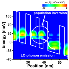
- Energy resolved local density of states (LDOS) (see Fig. in ICPS poster) (z, Ez,
LDOS(z,Ez))
in units of
[1 / (eVAngstrom)]
LocalDOS_avs.fld , *.coord, *.dat local density
of states (LDOS), i.e. real part of spectral function divided by 2pi at k||
= 0.
DOS_avs.dat
==> LDOS.v
spectral_real_avs.fld , *.coord, *.dat
(spectral_aimag_avs.fld, *.coord, *.dat)
-
spectral_real.dat
spectral_real2.dat:
spectral_aimag.dat:
spectral_aimag2.dat:
spectral_real_old.dat:
spectrum_ana.mtx: matrix representation of spectral_real.datspectrum_ana2.mtx: matrix representation of spectrum_aver.dat:
- Optical gain within linear response theory
These files contain the gain (and the absorption alpha
which is -gain)
gain(z,E) where z is the spatial
coordinate and E is the photon energy.
Note that positive values
correspond to gain, negative values to absorption.
The output units for the gain (i.e. -absorption) are [1/m].
- gain_Re.v
gain_Re.fld, *.coord, *.dat
(gain_Im.fld, *.coord, *.dat
==>
)
-
The x axis is the distance in units of [nm].
- The y axis is the photon energy in units of [eV].
The y axis is from
-
'min_photon' (minimum
photon energy relevant for gain) to
-
'max_photon' (maximum photon
energy relevant for gain) as specified in the input file.
-
'photon_number' (e.g. =
20, = 100)
is the number of energy grid steps between 'min_photon' and 'max_photon'.
- gain_integrated_energy.dat
contains the integrated gain over spatial coordinate divided
by interval used for integration:
gain(E)
where E is in units of [eV],
gain is in units [1/cm]
gain_integrated_wavelength.dat
contains the integrated gain over spatial coordinate divided
by interval used for integration:
gain(lambda) where lambda is in units of [µm],
gain is in units [1/cm]
Note: The interval that is used for integration is
specified via the optional flag:
 gain-integrate-device-from-to     =
5d0 65d0
! [nm]
- complex optical conductance sigma
optical_conductance_Re.fld, *.coord, *.dat: Re(sigma)
optical_conductance_Im.fld, *.coord, *.dat:
Im(sigma)
-
- The y axis is the photon energy in units of [eV].
The y axis is from
-
'min_photon' (minimum
photon energy relevant for gain) to
-
'max_photon' (maximum photon
energy relevant for gain) as specified in the input file.
-
'photon_number' (e.g. =
20, = 100)
is the number of energy grid steps between 'min_photon' and 'max_photon'.
The optical conductance is obtained from the quotient of the
perturbation of the current density delta j(z,w) and the electric field of
the photon Ez(w).
sigma(z,w) = delta j(z,w) / Ez(w)
- complex permittivity epsilon: epsilon(z,w) =
epsilon0 epsilonr(z) + i sigma(z,w)/w
[epsilon0]
dielectric_function_Re.fld, *.coord, *.dat: Re(epsilon)
dielectric_function_Im.fld, *.coord, *.dat:
Im(epsilon)
-
The x axis is the distance in units of [nm].
- The y axis is the photon energy in units of [eV].
The y axis is from
-
'min_photon' (minimum
photon energy relevant for gain) to
-
'max_photon' (maximum photon
energy relevant for gain) as specified in the input file.
-
'photon_number' (e.g. =
20, = 100)
is the number of energy grid steps between 'min_photon' and 'max_photon'.
Note: If the imaginary part of the dielectric function epsilon(z,w) is
negative, i.e. Im(epsilon) < 0, the medium delivers energy to the wave, and
thus amplifies the wave which corresponds to positive gain. If Im(epsilon) <
0, absorption is present.
Current (I-V characteristics)
IV_characteristics1D_NEGF.dat: current-voltage characteristics
(I-V characteristics)
There are three columns:
voltage[V] j_average[A/cm^2]
Deta_phi_electrostatic[V]
- applied bias: voltage in units of [V] - The
meaning of 'applied bias' is voltage difference between left and right
contact: applied_bias = Vleft - Vright = -(EF,left
- EF,right) / |e|.
- current density (averaged value over
all grid points (N-2)) in units of [A/cm2]
- difference in electrostatic potential of left and right
boundaries in units of [V]: Delta_phi = phi(1) - phi(Nz)
= phileft - phiright
The applied bias and Delta_phi have the same sign.
Here, one can check if the applied bias also drops in terms of electrostatic
potential drop.
An additional nonzero built-in potential (built-in-potential =
... in units of
[V]) has to be taken into account when comparing the electrostatic
potential drop to the applied bias.
Comments: If the conduction band edge at the left side is higher than
at the right side, then the electric field is negative.
Convergence files
During the calculation, one can check the status of the convergence.
minimum_ConductionBandEdge.dat: minimum of conduction band edge during iterations ==> if
converged, this value should be converged
Returns the lowest value (minimum) of the conduction band edge in units of [eV],
i.e. of the file
ConductionBandEdge_ind000.dat.
Note: min_potV is currently used only in FUNCTION
get_drift_momentum.convergence_density.dat: contains convergence parameter
for the density: relative change of
density with respect to previous iteration
These values are written out with
respect to the Poisson self-consistency cycle.
See also specifier
limit-for-density-convergence.convergence_density_temp.dat: contains convergence parameter
for the density: relative change of density with respect
to previous iteration
These values are written out in both the Poisson self-consistency
cycle and in the scattering self-consistency cycle.iterations_current.mtx: electron current density [A/Angstrom2]
- each line
corresponds to an iteration
- current density at each grid point (should be the same for
all grid points if converged)iterations_density.mtx: electron density
[1018 cm-3] - each line corresponds to an
iterationscreening_length_Debye.dat - electrostatic
Debye screening length in units of [nm]
screening_length_Lindhard.dat - electrostatic Lindhard
screening length in units of [nm] (The Lindhard screening length
is only an output quantity. It is not used inside the code.)
Both are written out in subroutine get_density.
The screening length is input for the computation of the
- lesser selfenergy due to inelastic scattering with LO-phonons.
- retarded and lesser selfenergy for elastic scattering on charged
impurities.
- retarded and lesser self-energies for the inelastic electron-electron
scattering. Here, the simplest approach for the screening is used: Debye
screening length
The Debye screening length is defined as
LD = SQRT ( epsilon0 * epsilonr
* kB T / (e2 n) )
where n is the averaged density in the device, i.e. a constant Debye
screening length is used.
See eq. (3.4.21), p. 54 in PhD thesis of T. Kubis.
Other files
tau.dat - test_greenL.dat - second_div_low.dat - LOS.dat - SUBROUTINE get_density
contains real part of the spectral function for k|| = 0.mass_nonparabolicity_avs.fld - energy and position
dependent effective mass in units of [m0], i.e. m(z,E) where E is the total
energy. alpha is the
nonparabolicity parameter.
m(z,E) = m(z) ( 1 + ( E - E_c(z) ) * alpha(z) )contact/contact_ElectrostaticPotential_left.dat - -electrostatic
potential at left contact, i.e. at leftmost grid point in units of [V]
contact/contact_ElectrostaticPotential_right.dat - -
Further output for debugging
$global-settings
...
debug-level = 2 ! Choose a
number higher than 0 for additional
output useful for debugging.
If the debug level is larger than 1, the following output is available:
debug/Greens_function_lesser(z,Ez,E).fld
lesser Green's function G<(z,z,Ez,E), i.e. G<(z,Ez,E)debug/Greens_function_retarded(z,Ez,E).fld retarded
Green's function GR(z,z,Ez,E), i.e. GR(z,Ez,E)
How to restart a calculation
If you used
save-every-nth-iteration =
3 ! saves information in binary format that can be read in
! later to restart a calculation (default:
10)
then you can restart a calculation by reading in previously saved
data. This feature is useful if you had a system crash or system shut down, for
instance. The calculations are then restarted from the point where the
NEGF/stop/*.raw files have been written.
- Generate a file named
run.txt in the folder of the
executable. The content of that file does not matter – it may be empty.
- Start the program with the same input file the
NEGF/stop/*.raw
files have been generated with.
- Wait until the following is written on the screen output, or in the
output file in the case you pipe (
> logfile.out) the screen
output (may take some time, depending on the job):
- reading the Green's functions
- reading the self-energies on hard drive
- reading the numerical constants
- reading the physical constants
- reading the remaining global variables
- reading the global functions
Then the reading of the former program process is done.
- Now you may delete the
run.txt file. That might be safer,
but it should not matter leaving the file as it is. (We have not seen any
problems with that.)
Note: If
save-every-nth-iteration =
1 is chosen, then for each iteration
the *.raw files are written. On modern architectures, this is
usually fast. On older systems, this might take significant time.
For an example of the Green's function functionality, have a look at the
RTD tutorial.
Parallelization of NEGF algorithm
The NEGF algorithm has been parallelized.
Two options for parallelization are available.
-
no parallelization
-
parallelization with
OpenMP (executables
compiled with Intel compiler, including parallel version of MKL)
Very easy to use, i.e. specify number of threads via command line:
nextnano3.exe -threads 4
(uses four threads, e.g. on a quad-core CPU)
For further details, see also:
$global-settings
...
number-of-threads = 2
! 2 = for dual-core CPU
Necessary input files
The following input files are necessary for the
NEGF algorithm. They are located in the folder input_files/NEGF/.
Recent changes
The following changes have been done for the 2012
version of nextnano³.
-
All output files related to the input
structure like conduction band edge profile, effective mass profile, ... are
now written to the folder NEGF/structure/.
-
All convergence files related to the
calculation are now written to the folder NEGF/convergence/.
convergence_density.dat was previously called
long_convergency.dat.
minimum_conduction_band_edge.dat was previously called
min_pot.dat.
-
Output files mapping_E.dat and
mapping_Ez.dat were previously called E_mappingV.dat and
Ez_mappingV.dat.
-
The output of the gain/absorption has now the
opposite sign, i.e. gain is positive, absorption is negative.
The integrated gain is now in units of [1/cm].
-
The specifier roughness_width in
the
$scattering-mechanisms section has been deleted. Now the position
dependent roughness width roughness_width should be specified
instead.
The specifier correlation_length in the
$scattering-mechanisms section has been deleted. Now the position
dependent roughness width correlation_length should be
specified instead.
Now the units are [nm] for both input and output. Previously
they were [Angstrom].
-
The following keywords and specifiers changed
slightly.
!------------------------------------------!
$nonparabolicity-profile
!
nonparabolicity = 1.5d0
! [1/eV]
start-point = 1
!
end-point = 95
!
$end_nonparabolicity-profile
!
!------------------------------------------!
-
The following specifiers are new:
get-alloy-from-nextnano = yes
mass-density
= ...
acoustic-deformation-potential = ...
-
limit-for-density-convergence
was previously called long_conv_limit.
Poisson-damping-threshold
poisson_limit.
zero-drift-vector-in-contacts zero_drift.
use-maximum-drift-vector
max_drift.
drift-vector-maximum [1/nm] drift_length [1/Angstrom]. Note that the
units have changed.
output-correlation-functions correlation.
output-quasi-Fermi-level
was previously called fermi.
output-k-resolved
was previously called k_resolved.
first-order-Born-approximation
was previously called first_born.
calculate-transmission
was previously called transmission.
Poisson-damping-1
was previously called poisson_damping1.
Poisson-damping-2
was previously called poisson_damping2.
Poisson-damping-3
was previously called poisson_damping3.
electric-field-at-contact-damping-1
was previously called slope_damping1.
electric-field-at-contact-damping-2
was previously called slope_damping2.
electric-field-at-contact-damping-3 slope_damping3.
scattering-self-energies-damping-1
self_damping1.
scattering-self-energies-damping-2 was previously called
self_damping2.
scattering-self-energies-damping-3 was previously called
self_damping3.
drift-vector-damping-1
was previously called drift_damping1.
drift-vector-damping-2
was previously called drift_damping2.
drift-vector-damping-3
was previously called drift_damping3.
alloy-scattering was previously called alloy_scattering.
lattice-constant was previously called lattice_constant.
acoustic-phonon-scattering was previously called
acoustic_phonons.
LO-phonon-scattering
optical_phonons.
electron-electron-scattering
electron_electron.
charged-impurity-scattering
was previously called charged_impurity.
interface-roughness-scattering was previously called
interface_roughness.
ballistic-calculation
ballistic.
contact-scattering-max-number-iterations was previously called
contact_scat.
contact-scattering-potential-broadening was previously called
contact_sc_pot.
fix-electric-field-at-contact
was previously called
given_slope.
electric-field-at-contact was previously called
poisson_slope.
electric-field-at-contact-limit was previously called
slope_limit.
built-in-potential
built_in_potential.
-
non_diagonal_range
is now in units of [nm]. Previously it was [Angstrom].
lattice-constant is now in units of [nm]. Previously it was [Angstrom].
sound-velocity is now in units of [m/s]. Previously it was [Angstrom/s].
electric-field-at-contact is now in units of [V/m]. Previously it was
called poisson_slope was in units of [V/Angstrom]
and had the opposite sign.
-
read-inputfile-during-calculation =
no ! default value is now:
no
To do:
-
Output gain_real_integrated_frequency.dat
alpha(nu)
-
Implement temperature
sweep.
-
Add alloy scattering
documentation to online docu and source code based on Jirauschek/Kubis
review article
This will become obsolete:
!--------------------------------------------------!
$doping-function-NEGF optional !
doping_density double required ! [1/Angstrom^3]
start_point integer optional !
end_point integer optional !
$end_doping-function-NEGF optional !
!--------------------------------------------------!
!--------------------------------------------------!
$potential-profile optional !
potential_height double required ! [eV]
start_point integer optional !
end_point integer optional !
$end_potential-profile optional !
!--------------------------------------------------!
!--------------------------------------------------!
$left-contact-potential-profile optional !
left_potential_height double optional ! [eV]
left_start_point integer optional !
left_end_point integer optional !
$end_left-contact-potential-profile optional !
!--------------------------------------------------!
!--------------------------------------------------!
$right-contact-potential-profile optional !
right_potential_height double optional ! [eV]
right_start_point integer optional !
right_end_point integer optional !
$end_right-contact-potential-profile optional !
!--------------------------------------------------!
!--------------------------------------------------!
$alloy-profile optional !
alloy_concentration double required ! []
alloy_pot_difference double optional ! [eV]
start_point integer optional !
end_point integer optional !
$end_alloy-profile optional !
!--------------------------------------------------!
!--------------------------------------------------!
$roughness-profile optional !
roughness_width double required ! [Angstrom]
correlation_length double optional ! [Angstrom]
start_point integer optional !
end_point integer optional !
$end_roughness-profile optional !
!--------------------------------------------------!
!--------------------------------------------------!
$mass-profile optional !
effective_mass double required ! [m0]
start_point integer optional !
end_point integer optional !
$end_mass-profile optional !
!--------------------------------------------------!
!--------------------------------------------------!
$nonparabolicity-profile optional !
nonparabolicity double required ! [1/eV]
start-point integer
optional !
end-point integer optional !
$end_nonparabolicity-profile optional !
!--------------------------------------------------!
!--------------------------------------------------!
$dielectric-profile optional !
dielectric_const double required ! []
dielectric_inf double required ! []
start_point integer optional !
end_point integer optional !
$end_dielectric-profile optional !
!--------------------------------------------------!
|