Output-kp-data
The output of the k.p eigenvalues and
eigenfunctions is controlled by this keyword. All eigenfunctions and eigenvalues
between vb-min-ev and vb-max-ev (for conduction band:
cb-min-ev and cb-max-ev) are written out in one
file.
!-------------------------------------------------------------!

$output-kp-data
optional !

 destination-directory
character
required !

 complex-wave-functions
character
optional !

 kp-spinors
character
optional !

 detailed-output
character
optional !

 scale
double
optional !

 shift-wavefunction-by-eigenvalue
character
optional !


!

 bulk-kp-dispersion
character
optional !


 bulk-kp-dispersion-3D
character


 optional
!

 grid-position

double_array
 optional !

 k-direction-from-k-point
double_array  optional !

 k-direction-to-k-point
double_array  optional !

 number-of-k-points
integer
optional !

 shift-holes-to-zero
 character
optional ! 'yes' / 'no'


!

 k-par-dispersion
character
optional !

 k-par-disp-ev-min
integer
optional !

 k-par-disp-ev-max
integer
optional !

 DOS-density-of-states
character
optional !

 DOS-Emin-Emax
double_array
optional ! [eV]

 DOS-points
integer
optional !


!

 !-------- range for eigenvalues and eigenfunctions
----------!


!

 cb-num-ev-min
integer
optional !

 cb-num-ev-max
integer
optional !

 cb-k-par-min
integer
optional ! 1D/2D

 cb-k-par-max
integer
optional ! 1D/2D

 cb-k-SL-min
integer
optional !
for superlattice
 cb-k-SL-max
integer
optional !
!

 vb-num-ev-min
integer
optional !

 vb-num-ev-max
integer
optional !

 vb-k-par-min
integer
optional ! 1D/2D

 vb-k-par-max
integer
optional ! 1D/2D

 vb-k-SL-min
integer
optional !
for superlattice
 vb-k-SL-max
integer
optional !
!

 interband-matrix-elements
character
optional !

 intraband-matrix-elements
character
optional !

 intraband-lifetime
character
optional !

 intraband-matrix-elements-operator
character
optional !


!

 optical-matrix-element-output
character
optional
!

 dipole-transition-type
character
optional
!

 initial-band-min
integer
optional
!

 initial-band-max
integer
optional
!

 final-band-min
integer
optional
!

 final-band-max

integer
optional
!


!

$end_output-kp-data
!

!-------------------------------------------------------------!
Syntax
destination-directory = kp/
Name of directory to which the files should be written. Must exist and
directory name has to include the slash (\ for DOS and / for UNIX).
complex-wave-functions = yes /
no    !
It would have been
better to call this amplitudes rather than
complex-wave-functions.
Flag whether to print out the wave functions psi (amplitudes) including real and
imaginary parts in addition to the output of the probability densities Psi².
If set to yes, then kp-spinors
is also set to yes.
kp-spinors = yes /
no
Flag whether to print out the n = 6 (6-band k.p) or n = 8 (8-band k.p)
k.p spinors Psii2 in
addition to the output of Psi² which is the sum of all six or eight spinors:
Psi² = SUMi=1n Psii2
Filename: 3Dkp8x8_spinori_el_qc001_kpar001_ev001.fld
/ *.coord / *.dat
 3Dkp8x8_spinori_complx_el_qc001_kpar001_ev001.fld
  /  *.coord   /  *.dat
(if complex-wave-functions = yes)
detailed-output = yes /
no
Flag whether to print out additional output for k.p.
In particular more information about the eigenvalues for each k||
vector.
scale        =
0.1d0
The scale parameter can be used to scale the size of the wave functions in
the output file.
This is just for visualization purposes in order to fit wavefunctions more
nicely into band structure plots. This scaling has no physical meaning.
So far, it scales the wave function psi and psi²
(i.e. the probability density) in the same way:
psi²' = scale * psi²

  psi'  = scale * psi
1D: The units of psi² are [1/nm], the units
of psi are SQRT([1/nm]).
This way the integrated psi² over the
whole device (which is in units of [nm]) equals 1.
2D: The units of psi² are [1/nm²], the units of psi
are SQRT([1/nm²]).
This way the integrated psi² over the
whole device (which is in units of [nm²]) equals 1.
3D: The units of psi² are [1/nm³], the units of psi
are SQRT([1/nm³]).
This way the integrated psi² over the
whole device (which is in units of [nm³]) equals 1.
(It holds for unscaled psi², i.e. scale = 1d0: A good check to see if psi² is
normalized correctly is to apply
Neumann boundary conditions at all boundaries of the quantum cluster. The
ground state probability density then is constant over the whole device. This
value in units of [1/nm] (1D), [1/nm²] (2D) or [1/nm³] (3D) multiplied by the
length (1D), area (2D) or volume (3D) of the quantum cluster must equal 1.)
shift-wavefunction-by-eigenvalue  = yes
!
(1D: yes
= default)
                                  =
no  !
no = default)
If yes, in addition to default output, the wave function psi and the
probability density psi2 are shifted with respect to their
eigenvalue.
This is sometimes useful when plotting the wave functions together with the
band edge profile.
The relevant output files have the label _shift in their file
names.
There are two different types of E(k) dispersion, i.e. energy vs. k
= (kx,ky,kz) vector plot:
- Bulk k.p dispersion (
bulk-kp-dispersion)
The bulk k.p is the dispersion E(kx,ky,kz)
of the material at a specific grid point (grid-position)
which can be a binary or ternary semiconductor.
These are the energy levels Ei of the 8-band k.p
Hamiltonian H(kx,ky,kz) which has the
dimension 8.
- k|| dispersion, i.e. kparallel
(
k-par-dispersion)
In contrast to the bulk k.p dispersion which refers to a
grid point, the k|| dispersion refers to the
whole quantum cluster.
1D simulation: The k|| dispersion is the dispersion
E(kx,ky) where z is the quantization direction, e.g.
for a quantum well grown along the z direction.
2D simulation: The k|| dispersion is the dispersion E(kz)
where x and y are the quantization directions, e.g. for a quantum wire
oriented along the z direction.
3D simulation: A k|| dispersion does not make sense.
These are the energy levels Ei of the 8-band k.p
Hamiltonian H(kx,ky,kz) which has the
dimension of 8 times the number of grid points in the structure.
Special case for superlattices
k|| dispersion, i.e. kparallel
(k-par-dispersion)
1D simulation: The k dispersion is the dispersion E(kx,ky,kSL)
where z is the quantization direction and the direction where periodic
boundary conditions are employed.
2D simulation: The k dispersion is the dispersion E(kSL,x,kSL,ykz)
where x and y are the quantization directions and the directions where
periodic boundary conditions are employed.
3D simulation: The k dispersion is the dispersion E(kSL,xL,kSL,yLkSL,z)
where x and y are the quantization directions and the directions where
periodic boundary conditions are employed.
These are the energy levels Ei of the 8-band k.p
Hamiltonian H(kx,ky,kz) which has the
dimension of 8 times the number of grid points in the structure.
Bulk k.p dispersion
See tutorial: k.p dispersion in bulk GaAs (strained / unstrained)
bulk-kp-dispersion = yes
!
Calculates energy dispersion E(k) where
k is real.
= real-and-imaginary-k-vector !
=
no
Flag that signals if you want to output the pure bulk k.p dispersion
E(k) = E(kx,ky,kz) along a line from
k = 0 to k = (kx,ky,kz).
This is especially of interest in strained regions where the bands are shifted
due to strain. The dispersion is taken at the material grid point grid-position
which has to be located inside a quantum region.
The parabolic, isotropic
dispersion of the effective-mass approximation (single-band) is included for
comparison.
bulk-kp-dispersion-3D = yes /
no

                      =
graphene   !
(special option for
bulk graphene tight-binding band structure)
Flag that signals if you want to put out the pure bulk k.p dispersion
E(k) = E(kx,ky,kz) over the
three-dimensional k space.
This can be of interest in strained regions where the bands are shifted due to
strain. The dispersion is taken at the material grid point grid-position
which has to be located inside a quantum region.
The maximum value kmax is determined by MAX(|k-direction-from-k-point|,|k-direction-to-k-point|).
k space grid resolution: The number of k points from the Gamma point
along each direction is number-of-k-points/4.
- bulk_8x8kp_dispersion3D_cb1.fld
  / *.dat / *.coord    / *_ijk.dat

  - bulk_8x8kp_dispersion3D_cb2.fld  / *.dat /
  *.coord    / *_ijk.dat

  - bulk_8x8kp_dispersion3D_hh1.fld  / *.dat /
  *.coord    / *_ijk.dat

  - bulk_8x8kp_dispersion3D_hh2.fld  / *.dat /
  *.coord    / *_ijk.dat

  - bulk_8x8kp_dispersion3D_lh1.fld  / *.dat /
  *.coord    / *_ijk.dat

  - bulk_8x8kp_dispersion3D_lh2.fld  / *.dat /
  *.coord    / *_ijk.dat

  - bulk_8x8kp_dispersion3D_soh1.fld / *.dat / *.coord
	/ *_ijk.dat

  - bulk_8x8kp_dispersion3D_soh2.fld / *.dat / *.coord
	/ *_ijk.dat
Note: The individual components are called
  cb1  = electron 1

          cb2
  = electron 2

          hh1
  = heavy     hole 1

          hh2
  = heavy     hole 2

          lh1
  = light     hole 1

          lh2
  = light     hole 2


  soh1 = split-off hole 1


  soh2 = split-off hole 2
which is correct ONLY for the unstrained case. In the
strained case the character is no longer "purely" heavy, light and
split-off hole-like if strain is present because all the states are mixed!
Note that the '1' and '2' states might be
degenerate.
grid-position = 20d0 ! in units of
[nm]
grid-position = 10d0
! x = 10 [nm]
(1D)

              =
10d0  20d0
! x = 10 [nm], y = 20 [nm]
(2D)

              =
10d0  20d0  20d0
! x = 10 [nm], y = 10 [nm], z = 20 [nm] (3D)
Determines position of point in structure for bulk dispersion
(must be within a k.p quantum cluster).
The bulk k.p dispersion can be calculated along
an arbitrary line from the k point 'k-direction-from-k-point'
to the Gamma point and then to the k point 'k-direction-to-k-point'.
Either k-direction-from-k-point or k-direction-to-k-point
or both can be zero. If both are zero, then only the Gamma point
is calculated.
If k-direction-from-k-point is omitted, then this specifier
takes the negative value of k-direction-to-k-point.
You can use this flag to specify a customized plot for the E(k)
dispersion, e.g. along a line from [110] to the Gamma point and then to the
[001] point.
k-direction-from-k-point = 0.0d0 1.0d0 1.0d0 ! [1/nm] along [011] direction with respect to
simulation coordinate system
            =
0.0d0  0.0d0  1.0d0
! [1/nm] [001] direction with respect to
simulation coordinate system
            =
- [k-direction-to-k-point]
  ! [1/nm]
(default, i.e. if k-direction-from-k-point is
omitted)
Determines k-direction and range for dispersion plot
[1/nm] to the Gamma point.
k-direction-to-k-point   = 0.0d0  1.0d0  1.0d0
  ! [1/nm]
along [011] direction with respect to
simulation coordinate system
            =
0.0d0 0.0d0 1.0d0 ! [1/nm] [001] direction with respect to
simulation coordinate system
            =
0d0    0d0    1d0          ! [1/nm]
(default, i.e. if k-direction-to-k-point is omitted))
Determines k-direction and range for dispersion plot
[1/nm] from the Gamma point.
number-of-k-points = 50 ! If
omitted, the default value of 50 is
used.
Number of k points to be calculated (resolution)
in addition to the Gamma point at (kx,kykz)
= (0,0,0) for the bulk k.p dispersion along a particular direction.
shift-holes-to-zero = yes


 = no
This is to shift the bulk dispersion curve, i.e. to set the zero point of
the energy axis to the topmost hole energy:
E(k=0) = 0 eV for the heavy and light holes
dispersion (unstrained case) or to the topmost hole energy (strained case or
wurtzite).
The conduction band dispersion then starts at the band gap energy and the
split-off energy dispersion at delta_split-off.
The strain can lift the degeneracy of heavy and light holes. Thus we define
for the zero of energy the topmost valence band energy if
shift-holes-to-zero = yes.
Output files
-
bulk_sg_dispersion000_kxkykz.dat
isotropic and parabolic
dispersion of single-band effective masses from [000] to [kx ky kz]
bulk_8x8kp_dispersion000_kxkykz.dat
-
bulk_sg_dispersion100_000_001.dat
isotropic and parabolic
dispersion of single-band effective masses from [100] to [000] to [001]
bulk_8x8kp_dispersion100_000_001.dat
bulk_8x8kp_dispersion110_000_001.dat dispersion of bulk
k.p Hamiltonian
from [110] to [000] to [001]
bulk_8x8kp_dispersion111_000_001.dat dispersion of bulk
k.p Hamiltonian
from [111] to [000] to [001]
These directions might not be general enough for wurtzite or strained structures
but one can rotate the crystal coordinate system with respect to the simulations
coordinate system accordingly in the input file.
Inside the code, the k.p Hamiltonian is calculated with respect
to the "calculation coordinate system" while it holds for all the output files
that the [kx,ky,kz] directions are related to
the "simulation coordinate system". So the software takes care of the rotations
automatically. Care has to be taken when analyzing the eigenvectors as the
quantization axis of spin is also relevant.
k|| dispersion
k-par-dispersion = no
!
no E(k||) dispersion
= yes !
                 =
01-00    !
= 01-00-11 !
= 01-00-10 ! E(k||)
= E(0,ky) dispersion for ky = [ky,max,...,0]
(where kx=0) and for
Flag that signals if you want to have the E(k||) = E(kx,ky) dispersion
to be put out. This is for the quantum mechanically calculated eigenvalues.
This also works for 2D (but then only no
and yes make
sense), i.e. E(kz) but does not make sense
for 3D.
'01-00', '01-00-11'
and '01-00-10'
are special options for slices along special
directions through the two-dimensional E(k||) = E(kx,ky)
dispersion.
- 01-00:
A plot of E(kx,ky) along the line from E(0,ky,max)
to E(0,0) .
- 01-00-11: A plot
of E(kx,ky) along the line from E(0,ky,max)
to E(0,0) (where kx=0) and along
the line from E(0,0) to E(kx,max,ky,max=kx,max)
for kx = ky
- 01-00-10: A plot
of E(kx,ky) along the line from E(0,ky,max)
to E(0,0) (where kx=0) and along the line from E(0,0)
to E(kx,max,0) (where ky=0)
Note: If you use k-par-dispersion = 01-00,
01-00-11
or 01-00-10, then the calculation is much
faster because only at the k|| points at these symmetry lines the
eigenvalues are calculated.
Obviously in this case you cannot do a
self-consistent calculation. Also plotting the 2D dispersion of E(kx,ky)
(i.e. the 2D plot) or the density of states is not correct in this case.
Specify the eigenvalue numbers (i.e. subband numbers) for which the energy
dispersion should be written out.
The following two specifiers do not distinguish between
electrons and holes.
k-par-disp-ev-min =  1

k-par-disp-ev-max = 10
Lower (min) and upper (max) boundary for range of eigenvalues
(ev) for which the k||
dispersion E(kx,ky) should be written out.
This also works for 2D, i.e. E(kz) but does not make sense
for 3D.
This specifier affects the energy dispersion plots E(k||), the
k||-space-resolved density plots n(kx,ky)
and the effective masses calculated from the dispersion.
This specifier can be used to output only the dispersion of the 1st
or 2nd subband and not the dispersion all of calculated subbands.
Density of states (DOS) for k|| dispersion
DOS-density-of-states = yes ! 'yes' / 'no'
flag to output the density of states (DOS) (default: 'no')
! only implemented for 1D so far, i.e. E(kx,ky)
 DOS-Emin-Emax         =
0d0  2.5d0 !
minimum
and maximum energy for density of states (DOS) [eV]
! used for DOS calculation
! for Monte Carlo part: used for DOS calculation and scattering tables
 DOS-points            =
1000       !
number of points between DOS-Emin and DOS-Emax (default: 1000).
! This number determines the grid resolution of the energy grid used for the density of states (DOS)
output.
           ==>
Energy_grid = (DOS_Emax - DOS_Emin) / DOS_Points = 2.5 eV / 1000 = 0.0025
eV
For more information on the output (e.g. units), see below.
For more information on the density of states, have a look at the tutorial:
Density of states (DOS) in a GaAs quantum well with infinite barriers
Conduction bands:
cb-num-ev-min = 1
Lower boundary for range of conduction band eigenvalues for which those and
the eigenfunctions are put out.
cb-num-ev-max = 1
Upper boundary for range of conduction band eigenvalues for which those and
the eigenfunctions are put out.
cb-k-par-min = 1
Lower boundary for range of conduction band k|| points in
1D for which
eigenvalues and eigenfunctions are put out.
Lower boundary for range of conduction band kz points in 2D for which
eigenvalues and eigenfunctions are put out.
(Does not make sense in 3D.)
cb-k-par-max = 1
Upper boundary for range of conduction band k|| points for which
eigenvalues and eigenfunctions are put out.
Upper boundary for range of conduction band kz points in 2D for which
eigenvalues and eigenfunctions are put out.
(Does not make sense in 3D.)
cb-k-SL-min = 1
Only for superlattices (should be greater than or equal to 1).
Lower bound for range of superlattice vectors Kz (1D),
Kx,Ky (2D), Kx,Ky,Kz
(3D).
cb-k-SL-max = 1
Only for superlattices (should be greater than or equal to 1).
Upper bound for range of superlattice vectors Kz
(1D), Kx,Ky (2D), Kx,Ky,Kz
(3D).
Valence bands:
vb-num-ev-min = 1
Lower boundary for range of valence band eigenvalues for which those and
the eigenfunctions are put out.
vb-num-ev-max = 1
Upper boundary for range of valence band eigenvalues for which those and
the eigenfunctions are put out.
vb-k-par-min = 1
Lower boundary for range of valence band k|| points in 1D for which eigenvalues and eigenfunctions are put out.
Lower boundary for range of valence band kz points in 2D for which
eigenvalues and eigenfunctions are put out.
(Does not make sense in 3D.)
vb-k-par-max = 1
Upper boundary for range of valence band k|| points in 1D for
which eigenvalues and eigenfunctions are put out.
Upper boundary for range of valence band kz points in 2D for which
eigenvalues and eigenfunctions are put out.
(Does not make sense in 3D.)
vb-k-SL-min = 1
Only for superlattices (should be greater than or equal to 1).
Lower bound for range of superlattice vectors Kz (1D),
Kx,Ky (2D), Kx,Ky,Kz
(3D).
vb-k-SL-max = 1
Only for superlattices (should be greater than or equal to 1).
Upper bound for range of superlattice vectors Kz (1D),
Kx,Ky (2D), Kx,Ky,Kz
(3D).
interband-matrix-elements = yes !
calculates interband matrix elements
=
no
==> square of spatial overlap matrix element | <psi_i* | psi_j>
|^2
The output files
interband1D_vb001_cb001_qc001_hlsg001_deg001_dir.dat
(heavy hole <-> Gamma conduction band)
interband1D_vb002_cb001_qc001_hlsg002_deg001_dir.dat
<-> Gamma conduction
band)
interband1D_vb003_cb001_qc001_hlsg003_deg001_dir.dat
<-> Gamma conduction band)
 Spatial overlap matrix elements | < psi_hl_i | psi_el_j > |^2 and


energy of transition in [eV]

 heavy hole <-> Gamma conduction band

------------------------------------------------------------------------

  |<psi_vb001|psi_cb001>|^2  0.987507995852382
1.654103

  |<psi_vb001|psi_cb002>|^2  1.336279027563441E-030

  |<psi_vb001|psi_cb003>|^2 -0.145559411422541
2.538366

  |<psi_vb002|psi_cb001>|^2  1.133344425625580E-030

  |<psi_vb002|psi_cb002>|^2 -0.964789984970279
2.065139
min-ev' to 'max-ev'.
To plot matrix elements vs. electric field.
 ('voltage-offset' + vbias) /
distance
with v_bias = sweep_index * sweep_voltage.
[kV/cm].
'voltage-offset' is the built-in potential in [V].
distance: lever-arm-length'.
MODULE bound_states_1D
must be initialized.
=> $quantum-bound-states
-> momentum matrix <psi*|p|psi> (not implemented yet)
-> Coulomb element <psi*|V|psi>
V = Int( 1/4pi (r1-r2) * |psi(r2)|‹dr2 )
intraband-matrix-elements-operator = "z^2" !
(needed for standard deviation)
= '0.0002 * x * ( x - 10)' !
$output-1-band-schroedinger
(not implemented yet)
intraband-matrix-elements = p
! < psif* | p
| psii >

                          =
z          ! < psif* | z
 | psii >

                          =
o          ! < psif* |       psii
>
(spatial overlap)
                          =
yes ! p' and
'z')
                          =
everything ! p',
'z', 'o',
and the one specified in intraband-matrix-elements-operator)
                          =
no         !
i means initial and f means
final state.
The output files
  intraband_p_cb1_qc1_6x6kp.txt


z
!
kind of matrix element ('p' / 'z'
/ 'o')
o
!
p' / 'z'
/ 'o')
vb1
!
cb001' /
heavy, light and split-off hole bands 'vb001')
8x8 !
6x6' / '8x8')
effective-mass') is counted
explicitely in k.p.
 | < psif* |
p | psii >
|
matrix element given in green color.)
-------------------------------------------------------------------------------

Intersubband transitions

=> Gamma conduction band

-------------------------------------------------------------------------------

Electric field in z-direction [kV/cm]: 0.0000000E+00

-------------------------------------------------------------------------------


-------------------------------------------------------------------------------

                   Intersubband dipole moment
| < psi_f* |
z | psi_i > |  [Angstrom]


       Intersubband dipole moment
| <
psi_f* | p | psi_i > |  [h_bar / Angstrom]

------------------|------------------------------------------------------------


Oscillator strength []

------------------|--------------|---------------------------------------------


Energy of transition [eV]

------------------|--------------|--------------|------------------------------


m* [m_0]

------------------|--------------|--------------|-----------|------------------

<psi001*|z|psi001>  249.0000
(matrix element <1|1> depends on choice of origin!)
<psi002*|z|psi001>
249.0000
(matrix element <2|1> depends on choice of origin!)
<psi001*|p|psi001>
1.8126842E-18
<psi002*|p|psi001> 1.8126842E-18
<psi003*|z|psi001>  18.01673
0.9602799      0.1694912  6.6500001E-02

<psi004*|z|psi001>  18.01673
0.9602799      0.1694912  6.6500001E-02

<psi003*|p|psi001>  2.6649671E-02  0.9602798
0.1694912  6.6500001E-02

<psi004*|p|psi001>  2.6649671E-02  0.9602798
0.1694912  6.6500001E-02


<psi005*|z|psi001>  3.5382732E-13

<psi006*|z|psi001>  3.5382732E-13

<psi005*|p|psi001>
2.1414240E-15

<psi006*|p|psi001>  2.1414240E-15


<psi007*|z|psi001>  1.441336
3.0698583E-02  0.8466209  6.6500001E-02

<psi008*|z|psi001>  1.441336
3.0698583E-02  0.8466209  6.6500001E-02

<psi007*|p|psi001>  1.0649348E-02  3.0698583E-02
0.8466209  6.6500001E-02

<psi008*|p|psi001>  1.0649348E-02  3.0698583E-02
0.8466209  6.6500001E-02


<psi009*|z|psi001>
7.2598817E-13

<psi010*|z|psi001>  7.2598817E-13

<psi009*|p|psi001>
1.0445775E-14

<psi010*|p|psi001>  1.0445775E-14


<psi011*|z|psi001>  0.3971008
5.4281550E-03  1.972205   6.6500001E-02

<psi012*|z|psi001>  0.3971008
5.4281550E-03  1.972205   6.6500001E-02

<psi011*|p|psi001>  6.8347319E-03  5.4281550E-03
1.972205   6.6500001E-02

<psi012*|p|psi001>  6.8347319E-03  5.4281550E-03
1.972205   6.6500001E-02


 ...

<psi039*|z|psi001>  1.0178294E-02
3.9452352E-05  21.81846   6.6500001E-02

<psi040*|z|psi001>  1.0178294E-02  3.9452352E-05
21.81846   6.6500001E-02

<psi039*|p|psi001>  1.9380630E-03  3.9452349E-05
21.81846   6.6500001E-02

<psi040*|p|psi001>  1.9380630E-03  3.9452349E-05
21.81846   6.6500001E-02


Sum rule of oscillator strength: f_j,001 = 0.9994023

Sum rule of oscillator strength: f_j,001 = 0.9994023

  ...
| Mfi | = | integral (psif* (z) z psii
(z) dz) |
and the oscillator strengths
ffi = 2m* / hbar² (Ef
- Ei) | Mfi |²
between all calculated
states in each band from eigenvalues 'min-ev' to 'max-ev'.
Unfortunately, the commonly used
Intersubband dipole moment  | < psi_f* | z | psi_i > |
[Angstrom]
depends on the choice of origin for the matrix elements where f = i
(also f+1 = i in some cases because of spin degeneracy, see above), thus the user might prefer to output the
Intersubband dipole moment  | < psi_f* | p | psi_i > |
[h_bar / Angstrom]
which are the intersubband dipole moments
| Nfi | = | integral (psif* (z) pz psii
(z) dz) | = | - i hbar integral (psif* (z) d/dz psii
(z) dz) |
and the oscillator strengths
ffi = 2m* / hbar² (Ef
- Ei) | Mfi |² = 2
/ ( m* (Ef
- Ei) ) | Nfi |²
between all calculated
states in each band from eigenvalues 'min-ev' to 'max-ev'.
For more details, have a look at the tutorial:
Optical
intersubband transitions in a quantum well - Intraband matrix elements and selection rules
intraband-lifetime = yes !
calculates the lifetime of intersubband transitions
= no ! does nothing
(default)
This feature is useful for e.g. quantum cascade lasers.
Note: intraband-matrix-elements must not be set to no
in order to print out the lifetimes (scattering rates).
See tutorial "Scattering times for electrons in unbiased and biased single and multiple
quantum wells" for more details.
Output:
Simple files (eigenvalues and square of the wave functions)
kp_8x8eigenvalues_qc001_el_kpar0005_1D_dir.dat
kp_8x8eigenvalues_qc001_el_kpar0005_1D_dir_info.dat
contains all electron eigenvalues for k = 0 and quantum cluster 1
for k|| vector 5.
Similar for holes and 6-band k.p.
The file with the suffix _info contains information about the
character of the eigenvalues, i.e. their S-like, heavy-hole, light-hole and
split-off hole character.
num_ev energy[eV] P_CB   P_HH
	P_LH   P_SO    sum
	P_CB1  P_CB2  |3/2,3/2> |3/2,-3/2> |3/2,1/2>
	|3/2,-1/2> |1/2,1/2> |1/2,-1/2>

	1      0.1678     0.7543 0.0000
	0.2208 0.02482 1.0000    0.7543 0.0000 0.0000
	0.0000     0.2208    0.0000
0.02482 0.0000kp_8x8psi_squared_qc001_el_kpar0005_1D_dir.dat
kp_8x8psi_squared_qc001_el_kpar0005_1D_dir_shift.dat
-
Note that in this file psi2
is shifted by the corresponding eigenvalues so that the square of the
wave functions can be plotted into the conduction/valence band edge diagram.
Similar for holes and 6-band k.p.
dir = Dirichlet boundary conditions
neu = Neumann boundary conditions
per = periodic boundary conditions
k.p eigenvalues
e.g. kp_8x8eigenvalues_pos_qc001_el_kpar0001_1D_dir.dat
This file contains all eigenvalues. It can be plotted into a conduction or
valence band profile diagram. Note that this file is written out only if
detailed-output = yes.
k.p eigenfunctions
Filename:
kp_8x8_el1D_wv_qc001_ev003_kpar001_Kz001_dir.dat |
8x8 |
|
|
|
|
|
|
Kind of kp solved (8-band or
6-band) |
| |
_el1D_wv |
|
|
|
|
|
Electron/hole (_el/_hl)
eigenvectors (_wv) |
| |
|
_qc001 |
|
|
|
|
Number of quantum cluster |
| |
|
|
_ev001 |
|
|
|
Number of eigenvalue |
| |
|
|
|
kpar001 |
|
|
Number of k|| point |
| |
|
|
|
|
Kz001 |
|
Number of Kz point
(superlattice vector) |
| |
|
|
|
|
|
_dir |
Boundary condition: Neumann/Dirichlet (_neu/_dir) |
Structure:
| position[nm] |
PSI^2_SUM |
PSI^2(1) |
PSI^2(2) |
PSI^2(3) |
PSI^2(4) |
PSI^2(5) |
PSI^2(6) |
PSI^2(7) |
PSI^2(8) |
| Position |
Sum of components^2 |
Squares of components of k.p-vector.
Eight in case of 8-band k.p / six for 6-band k.p. |
k.p complex eigenfunctions:
Filename:
kp_comp_8x8_el1D_wv_qc001_ev002_kpar001_Kz001_dir.dat |
_comp |
|
|
|
|
|
|
|
Complex wave functions |
| |
_8x8 |
|
|
|
|
|
|
Kind of k.p solved (8-band or
6-band) |
| |
|
_el1D_wv |
|
|
|
|
|
Electron/hole (_el/_hl)
wavevectors (_wv) |
| |
|
|
_qc001 |
|
|
|
|
Number of quantum cluster |
| |
|
|
|
_ev001 |
|
|
|
Number of eigenvalue |
| |
|
|
|
|
kpar001 |
|
|
Number of k|| point |
| |
|
|
|
|
|
Kz001 |
|
Number of Kz point
(superlattice vector) |
| |
|
|
|
|
|
|
_dir |
Boundary condition:
Neumann/Dirichlet (_neu/_dir) |
Structure:
| position[nm] |
PSI_real001 |
PSI_imag001 |
... |
| position |
Real part of 1st component |
Imaginary part of 1st component |
... |
schroedinger-kp-discretization = box-integration
The eight spinor components of the 8-band k.p wave function are
(for zinc blende): |
cb+ >, | cb- >, | hh1+ >, | lh1 >, | lh2 >, | hh2- >, | so1 >,
| so2 >
cb = conduction band
hh =
lh =
so =
+ = spin up
- = spin up
+ and - correspond to the spin projection along the z
axis of the crystal system ( + = up, - = down).
Note that the states | lh1 >, | lh2 >, | so1 >,
| so2 > are a mixture of spin up and spin down.
|  J ,   m  >

  | 3/2,  3/2 >  =  | hh1+ >

  | 3/2,  1/2 >  =  | lh1  >

  | 3/2, -1/2 >  =  | lh2  >

  | 3/2, -3/2 >  =  | hh2- >

  | 1/2,  1/2 >  =  | so1  >

  | 1/2, -1/2 >  =  | so2  >
schroedinger-kp-discretization =
	box-integration-XYZ


	=
  finite-differences
The eight spinor components of the 8-band k.p wave function are
(for zinc blende): |
cb+ >, | cb- >, | x+ >, | y+ >, | z+ >, | x- >, | y- >, | z- >
| x >, | y >, | z > correspond to x, y, z of the calculation
system.
Note: In nextnano3 k.p subroutine we introduced an
unnecessary rotation. When we get rid of it in the future, we will have |
x >, | y >, | z > in crystal system. kx, ky are in calculation system.
For more details, see eq. (3.85) in the
PhD thesis of S. Birner.
k.p bulk dispersion:
Bulk k.p dispersion E(k).
Filename:
bulk_8x8kp_dispersion000_kxkykz.dat (k.p dispersion)
bulk_sg_dispersion000_kxkykz.dat
Structure:
| k |
hi ( i = 1-8, or 1-6) |
Position in k space in direction of k-direction-to-k-point [1/nm] |
Eigenvalues of bulk k.p Hamiltonian |
See tutorial: k.p dispersion in bulk GaAs (strained / unstrained)
k|| dispersion:
Remark:
1D: The output is two-dimensional because the dispersion in the whole plane
perpendicular to the quantization direction is calculated. The output therefore
consists of three files (AVS/Express format):
AVS/Express
Field file: kpar1D_disp_hl_6x6kp_qc001_ev001_2Dplot.fld
AVS/Express field file
Coordinates: kpar1D_disp_hl_6x6kp_qc001_ev001_2Dplot.coord
AVS/Express coordinate files, x/y coordinates
Data file:
kpar1D_disp_hl_6x6kp_qc001_ev001_2Dplot.dat
AVS/Express data file, dispersion in nonquantized
directions
Filename:
kpar1D_disp_hl_6x6kp_qc001_ev001_2Dplot.dat |
_hl/_el |
|
|
File containing data for conduction band
(_el) or valence band (_hl) eigenstates |
| |
_6x6kp/_8x8kp |
|
kind of k.p (6-band or 8x8) |
| |
_qc001
|
|
Number of quantum cluster |
| |
|
_ev001 |
Number of eigenvalue of subband |
Structure:
| E_val_k_par: |
| Eigenvalues of k|| points |
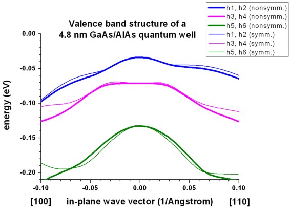
Example: See Tutorial "Energy dispersion of holes in quantum wells".
k||
dispersion from [00] to [10]:
1D: This file contains data of a cut along the line from zero (i.e. [kx,ky]
= [0,0] = [00]) to [10] (i.e. [kx,ky] = [kx,0]
where kx > 0) of the 2D plot of the E(k||)=E(kx,ky)
dispersion.
Filename:
kpar1D_disp_00_10_hl_6x6kp_ev001.dat

kpar1D_disp_00_10_el_8x8kp_ev001.dat
kpar1D_disp_00_10_hl_6x6kp_ev001.dat |
_hl/_el |
|
|
File containing data for conduction band
(_el) or valence band (_hl) eigenstates |
| |
_6x6kp/_8x8kp |
|
kind of k.p (6-band or 8x8) |
| |
|
_ev001 |
Number of eigenvalue of subband |
Structure:
abscissa |
eigenvalue |
kx |
ky |
num_kpar |
kx |
Eigenvalue of k|| point |
kx position [1/Angstrom] |
ky position [1/Angstrom] |
Number of k|| point |
The file kpar1D_disp_00_10hl_8x8kp_ev_min001kp_ev_max010.dat
contains essentially the same data but here all subband dispersions from
eigenvalue min001 to eigenvalue max011 are contained
in one single file.
k||
dispersion from [01] to [00] and from [00] to [11]:
1D: This file contains data of cuts along the line from [01] to zero
and from zero to [11] of the 2D plot of the E(k||)=E(kx,ky)
dispersion.
Filename:
kpar1D_disp_01_00_11_hl_6x6kp_ev001.dat

kpar1D_disp_01_00_11_el_8x8kp_ev001.dat
kpar1D_disp_01_00_11_hl_6x6kp_ev001.dat |
_hl/_el |
|
|
File containing data for conduction band
(_el) or valence band (_hl) eigenstates |
| |
_6x6kp/_8x8kp |
|
kind of k.p (6-band or 8x8) |
| |
|
_ev001 |
Number of eigenvalue of subband |
Structure:
abscissa |
eigenvalue |
kx |
ky |
num_kpar |
-ky
    -- for [01] to [00]

SQRT(kx²+ky²) -- for [00] to [11] |
Eigenvalue of k|| point |
kx position [1/Angstrom] |
ky position [1/Angstrom] |
Number of k|| point |
To plot the data file, only the first (abscissa) and the second column
(eigenvalue) are important.
Example: See Tutorial "Energy dispersion of holes in quantum wells".
The file kpar1D_disp_01_00_11hl_8x8kp_ev_min001kp_ev_max010.dat
contains essentially the same data but here all subband dispersions from
eigenvalue min001 to eigenvalue max011 are contained
in one single file.
Simple
k||
dispersion data:
Filename:
kpar1D_disp_simple_hl_6x6kp_ev001.dat

kpar1D_disp_simple_el_8x8kp_ev001.dat
kpar1D_disp_simple_hl_ev001.dat |
_hl/_el |
|
|
File containing data for conduction band
(_el) or valence band (_hl) eigenstates |
| |
_6x6kp/_8x8kp |
|
kind of k.p (6-band or 8-band) |
| |
|
_ev001 |
Number of eigenvalue of subband |
Structure:
num_kpar |
kx |
ky |
eigenvalue |
| Number of k|| point |
kx position [1/Angstrom] |
ky position [1/Angstrom] |
Eigenvalue of k|| point |
This file cannot be plotted. It just contains for each k||
point the corresponding kx and ky values as well as its
corresponding eigenvalue.
Density of states (DOS)
The two-dimensional density of states (DOS) is written to the files 'DOS_hl_6x6kp.dat'
and 'DOS_hl_6x6kp_sum.dat' (and similar for electrons).
The DOS has been calculated from the energy dispersion E(k) = E(kx,ky).
'DOS_hl_6x6kp_norm.dat'
=======================
This file contains the density of states (DOS) for each eigenvalue (i.e.
subband).
The first column contains the energy in units of [eV], the other columns the
DOS of each individual subband in units of [eV-1 m-2].'DOS_hl_6x6kp_sum_norm.dat'
===========================
This file contains the density of states (DOS) , summed over each
eigenvalue (i.e. subband).
The first column contains the energy in units
of [eV], the second column the DOS (sum over all subbands) in units of [eV-1
m-2].
For the above two files, the x axis is in units of [eV] and its boundaries can be
adjusted by the following specifier:
DOS-Emin-Emax = 0d0 2.5d0 ! [eV]
The energy grid of the x axis (energy grid resolution) can be adjusted by the
following specifier which determines the
number of points between DOS-Emin and DOS-Emax:
DOS-points    = 1000

==>  Energy_grid = (DOS_Emax - DOS_Emin) / DOS_Points = 2.5 eV / 1000
= 0.0025 eV
The files Density_at_energy_el.dat and
Density_at_energy_hl.dat contain the energy resolved density n(E).
n(E) = DOS(E) * f(E) where f(E) is the Fermi function and DOS(E) is the density
of states at energy E.
energy[eV] n(E)[eV^-1cm^-2]
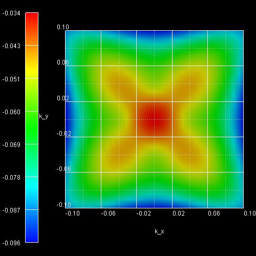
Density n(kx,ky)
kpar1D_density_el_8x8kp_qc001_2Dplot.fld
-
contains density as a function of kx and ky: n(kx,ky)
kpar1D_density_el_8x8kp_qc001_ev001_2Dplot.fld - contains
density as a function of kx and ky: ni(kx,ky)
for each eigenvalue i
The units are dimensionless, i.e. if one integrates over kx and ky
(which are in units of [1/m]), one gets a sheet charge density in
units of [m-2].
Optics
For the option to calculate and output the optical
matrix elements we need the following specifiers.
 optical-matrix-element-output = no


= yes       !
output of intensity, oscillator strength and transition energies
= complex !
 dipole-transition-type        =
el-el


= el-hl


= hl-el


= hl-hl

 initial-band-min
= 1

 initial-band-max
= 2

 final-band-min
= 8

 final-band-max
= 9
Note: For 'el-hl' initial means 'el',
final means 'hl'.
hl-el'
initial means 'hl', final means 'el'.
Example: In this example, the following transitions are considered:
     1 ->
8

     1 ->
9

     2 ->
8

     2 ->
9
1D:
This generates a 2D plot (in the AVS/Express format) for the intensity I(kx, ky)
in units of [eV].
In addition, a 2D plot for the optical matrix
element: P(kx, ky) in units of SQRT([2eV/m0])
is generated if optical-matrix-element-output =
complex.
Note that the intensity and the matrix element are
three-dimensional vectors with components Ix, Iy, Iz
or Px, Py, Pz, respectively, and kx, ky
is in units of [1/nm].
The optical matrix element will be calculated between band-min and
band-max eigenvalues.
The k|| points are the same that are chosen for the energy
dispersion output.
Output units:
a) Intensity: I = 2/m0 * |<
e.P >|2: Ix, Iy, Iz, Ixy,
Ixz, Iyz in units of
[eV] where Ii = 2/m0 |Pi|2,
Iij = 2/m0 |Pij|2 (i=x,y,z;
j=1,2,3).
b) complex value of the momentum matrix element Px, Py, Pz, Pxy, Pxz, Pyz
in units of
SQRT([2eV/m0]).
e is the light polarization vector
P is the momentum operator (vector)
Px(k) = <psi1(k)| e.P |psi2(k)>, where |e|=1,
e || x (i.e. e || [1,0,0], (x
polarization))
Pxy(k) = <psi1(k)| e.P |psi2(k)>, where |e|=1,
e || xy (i.e. e || [1,1,0], (xy
polarization))
The file 'opt_Intensity_info...txt' contains the
following data:
optical-matrix-element-output = yes
! [eV]
kx[1/nm] ky[1/nm] kz[1/nm]
Ix
Iy
Iz
Ixy
Ixz
Iyz
The file 'opt_MatrixElement_info...txt' contains the
following data:
 optical-matrix-element-output =
complex
! Units: SQRT([2eV/m0])
kx[1/nm] ky[1/nm] kz[1/nm] Re(Px)
Im(Px) Re(Py) Im(Py) Re(Pz)
Im(Pz) Re(Pxy)
Im(Pxy) Re(Pxz) Im(Pxz) Re(Pyz)
Im(Pyz)
Optical oscillator strength
|
 |
|
Example: Optical oscillator strength
of the fundamental transition in a 2D quantum wire calculated by 8-band k.p theory. The optical matrix elements (complex)
were calculated. In the picture one can see the dependence on the
polarization.
Note that the
oscillator strength is a dimensionless quantity. It is useful in order to
compare the probabilities of different dipole transitions.
(The calculations were
performed by Michael Povolotskyi, University of Rome "Tor Vergata".) |
Most attention is paid to
the matrix element. It is not taken from the database (or input file), instead
it is calculated from the k.p Hamiltonian.
Due to this approach all kinds
of dipole transitions are calculated in the same manner. All the symmetry is
taken into account automatically.
Example: Optical intraband TE mode (transverse electric) transitions are treated
correctly within k.p.
(Note that they are not zero within k.p but
they are zero for electrons in a single band approach.)
k.p material parameters
The k.p material parameters can be found
in the folder material_parameters/.
The file 6x6kp_parameters1D_used.dat
contains the following columns:
material_grid
[nm] on material grid
L M N+ N- N
6-band k.p Dresselhaus parameters L,M,N. Note: N = N+
+ N-
This file
6x6kp_Luttinger_parameters1D_used.dat contains the following columns:
material_grid
position in [nm] on material grid
gamma1 gamma2 gamma3 (kappa)
kappa is not used, it is in brackets)
(A) (B) (C^2)
[hbar2/2m0],
Phys. Rev. 98, 368 (1955)
The dispersion is nonparabolic if both B and C are nonzero.
(m_hh_iso) (m_lh_iso) (m_so_iso)
A. Baldereschi, N.O. Lipari, PRB 8, 2697 (1973)
(m_hh_100) (m_lh_100)
(m_hh_110) (m_lh_110)
(m_hh_111) (m_lh_111)
The A, B, C parameters and the masses are
currently not used inside the code. These values are just calculated and printed
out to make the k.p parameters "more transparent".
If it holds
gamma2 = gamma3 (spherical approximation) then the valence
band energy dispersion is isotropic. (This is equivalent to: L - M = N.)
|