|
| |
nextnano3 - Tutorial
next generation 3D nano device simulator
1D Tutorial
k.p dispersion in bulk unstrained ZnS, CdS, CdSe and ZnO (wurtzite)
Author:
Stefan Birner
If you want to obtain the input files that are used within this tutorial, please
check if you can find them in the installation directory.
If you cannot find them, please submit a
Support Ticket.
-> bulk_6x6kp_dispersion_ZnS_nn3.in

-> bulk_6x6kp_dispersion_CdS_nn3.in

-> bulk_6x6kp_dispersion_CdSe_nn3.in

-> bulk_6x6kp_dispersion_ZnO_nn3.in  / *_nnp.in -
input file for nextnano3
/ nextnano++ software
k.p dispersion in bulk unstrained ZnS, CdS, CdSe and ZnO (wurtzite)
This tutorial is based on
Valence band parameters of wurtzite materials
J.-B. Jeon, Yu.M. Sirenko, K.W. Kim, M.A. Littlejohn, M.A. Stroscio
Solid State Communications 99, 423 (1996)
- We want to calculate the dispersion E(k) from |k|=0 [1/nm] to |k|=2.0
[1/nm] along the
following directions in k space:
- [000] to [0001], i.e. parallel to the c axis (Note: The c axis is parallel
to the z axis.)
- [000] to [110], i.e. perpendicular to the c axis (Note: The (x,y) plane is
perpendicular to the c axis.)
We compare 6-band k.p theory results vs. single-band (effective-mass)
results.
- We calculate E(k) for bulk ZnS, CdS and CdSe (unstrained).
Bulk dispersion along [0001] and [110]
  $output-kp-data

 destination-directory  = kp/


 bulk-kp-dispersion     = yes

   grid-position          =
	5d0
	!
in units of [nm]
 !-----------------------------------------------------------------------------------

 ! Dispersion along [001] direction, i.e.
	parallel      to c=[0001] axis in wurtzite

 ! Dispersion along [110] direction, i.e.
	perpendicular to c=[0001] axis in wurtzite

 ! maximum |k| vector = 2.0 [1/nm]

 !-----------------------------------------------------------------------------------

 k-direction-from-k-point = 0d0
	0d0          2.0d0 !
k-direction and range for dispersion plot [1/nm]
k-direction-to-k-point = 1.41421356d0
1.41421356d0 0d0 ! k-direction and range for
dispersion plot [1/nm]
! The dispersion is calculated from the k point 'k-direction-from-k-point'
to Gamma, and then from the Gamma point to 'k-direction-to-k-point'.
number-of-k-points = 100 !
$end_output-kp-data- We calculate the pure bulk dispersion at
grid-position=5d0,
i.e. for the material located at the grid point at 5 nm. In our case this is
ZnS but it could be any strained alloy.
In the latter case, the k.p
Bir-Pikus strain Hamiltonian will be diagonalized.
The grid point at grid-position must be located inside a quantum cluster.
shift-holes-to-zero = yes forces the
top of the valence band to be located at 0 eV.
How often the bulk k.p Hamiltonian should be solved can be specified
via number-of-k-points. To increase the resolution, just increase
this number.
- The maximum value
of |k| is 2.0 [1/nm].
Note that for values of |k| larger than 2.0
[1/nm],
k.p theory might not
be a good
approximation any more.
This depends on the material system, of course.
- Start the calculation.
The results can be found in:
kp_bulk/bulk_6x6kp_dispersion_as_in_inputfile_kxkykz_000_kxkykz.dat
kp_bulk/bulk_sg_dispersion.dat (single-band approximation)
bulk_6x6kp_dispersion_as_in_inputfile_kxkykz_000_kxkykz.dat:
The first column contains the |k| vector in units of [1/nm], the next six
columns the six eigenvalues of the 6-band k.p Hamiltonian for this
k=(kx,ky,kz) point.
The resulting energy dispersion is usually discussed in terms of a
nonparabolic and anisotropric energy dispersion of heavy, light and
split-off holes, including valence band mixing.
bulk_sg_dispersion.dat:
The first column contains the |k| vector in units of [1/nm], the next
three columns the energy for heavy (A), light (B) and crystal-field
split-off (C) hole for this k=(kx,ky,kz)
point.
The single-band effective mass dispersion is parabolic and depends on a
single parameter: The effective mass m*.
Note that in wurtzite materials, the mass tensor is usually anisotropic with
a mass mzz parallel to the c axis, and two masses perpendicular
to it mxx=myy.
Results
- Here we visualize the results.
The final figures will look like this (left: dispersion along [0001], right:
dispersion along [110]):
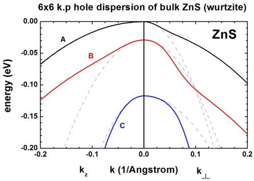
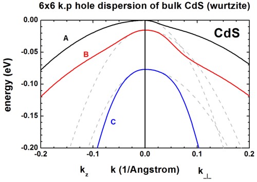
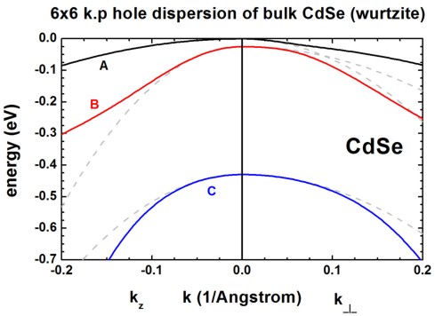
- These three figures are in excellent agreement to Figure 1 of the paper by [Jeon].
- The dispersion along the hexagonal c axis is substantially different than
the dispersion in the plane perpendicular to the c axis.
The effective mass approximation is indicated by the dashed, grey lines.
For the heavy holes (A), the effective mass approximation is very good
for the dispersion along the c axis, even at large k vectors.
- For comparison, the single-band (effective-mass) dispersion is
also shown. For ZnS, it corresponds to the following effective hole masses:
	 valence-band-masses = 0.35d0  0.35d0
2.23d0 ! [m0] 2.23 along c axis)
0.485d0 0.485d0 0.53d0 ! [m0]
0.53 along c axis)
0.75d0 0.75d0 0.32d0 ! [m0]
0.32 along c axis)
One can
see that for |k| < 0.5 [1/nm] the single-band approximation is in
excellent agreement with 6-band k.p but
differs at larger |k| values substantially.
- Plotting E(k) in three dimensions
Alternatively one can print out the 3D data field of the bulk E(k) =
E(kx,ky,kz) dispersion.
	$output-kp-data
  ...
  bulk-kp-dispersion-3D  =
	yes


	!----------------------------------------
! maximum |k| vector =
	2.0 [1/nm]
!----------------------------------------
  k-direction-to-k-point =
  	0d0  0d0 2.0d0   !
k-direction
and range for dispersion plot [1/nm]
number-of-k-points =
40
!
number of k points to calculated (resolution)
The meaning of number-of-k-points =
41
is the following:
40 k points from '- maximum |k| vector'
to zero (plus the Gamma point) and
40 k points from zero to '+ maximum |k| vector'
(plus the Gamma point)
along all three directions,
i.e. the whole 3D volume then contains 81 * 81 * 81 = 531441
k points.
k.p dispersion in bulk unstrained ZnO
The following figure shows the bulk 6-band k.p energy dispersion for ZnO.
The gray lines are the dispersions assuming a parabolic effective mass.
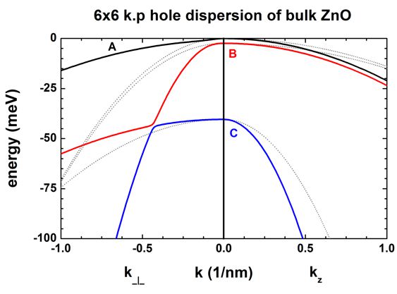
The following files are plotted:
- kp_bulk/bulk_6x6kp_dispersion_as_in_inputfile_kxkykz_000_kxkykz.dat

- kp_bulk/bulk_sg_dispersion.dat
The files
- bulk_6x6kp_dispersion_axis_-100_000_100.dat
- bulk_6x6kp_dispersion_diagonal_-110_000_1-10.dat
contain the
same data because for a wurtzite crystal, due to symmetry, the dispersion in the
plane perpendicular to the kz direction (corresponding to
[0001]) is isotropic.
|